The Fourth Operation

Use Ctrl + or – to enlarge or reduce text size.

The Fourth Operation
- tetration from a real perspective -
Introduction · Groping for a Solution · Uniqueness · A Related Problem · Facts About Functions · Asymptotic Power Series · To Proceed · The Original Problem · Computer Program I · Another Path · Computer Program II · Is it Unique? · Bases Other Than e · Review and Complex Numbers · A Zero’th Operation? · Other Terminology and Notation · Afterword

Introduction
Given whole numbers A and B we can add them together to get another whole number,

A + B

The definition of this operation is simply to count together what A and B count separately.

Then we can define multiplication as repeated addition:

A · B =	A + A + A + ...
	B times

And exponentiation as repeated multiplication:

A^{^B} =	A · A · A · ...
	B times

Those are the first, second, and third operations: addition, multiplication, and exponentiation. Presented in this manner a prolonged series of operations comes to mind, each operation iterating the one before. The fourth operation would be (using a subscript to denote the second operand):

A_{_B} =	A^{^A}^{^{^{^A}}}^{^{^{^{^···}}}}
	B times

We chose the grouping of the tower of A’s so that the exponentiations are done from top to bottom, A to the (A to the (A to the ...)). Any other grouping would collapse, at least in spots, reverting to the third operation, because (X to the X) to the Y equals X to the (X·Y).

The series of operations can be defined recursively on the second operand.

Addition:

Given.

Multiplication:

A · 1 = A

A · (B + 1) = A + A · B

Exponentiation:

A^¹ = A

A^{^{B + 1}} = A · A^{^B}

The fourth operation:

A_₁ = A
A_{_{B + 1}} = A^{^A_{_B}}

The n^th operation, for n > 1:

A [n] 1 = A

A [n] (B + 1) = A [n – 1] ( A [n] B )

Historical note: A [n] B when A and B are whole numbers is the same as the function φ(A, B, n – 1) of Wilhelm Ackermann (1896 – 1962), used in a paper of 1928.

Thus we can define a series of operations between positive whole numbers. It is well known how to extend the definition of the first two operations, addition and multiplication, to include all real numbers. The third, exponentiation, can be substantially so extended. The only restriction is that the base, A in A^{^B}, be nonnegative; this is necessary to ensure that the operation is well-defined and continuous as the exponent, B, varies.

The problem we investigate here is how to define the fourth operation, A_B or A raised to itself B times, for fractional B. What, for example, is A_½ or A raised to itself one half times? It might sound like a crazy question but no crazier than asking what is A multiplied by itself one half times. In that case the answer is the square root of A.

For now, it will make some formulas simpler if we consider just the case A = e, the base of the natural logarithms.

e₀ = 1
e₁ = e = 2.71828…
e₂ = e^e = 15.15426...
e₃ = e^e^{^e} = 3814279.10476…
etc.

What is

e_s

when s is not a whole number?

In order to solve the problem we will reformulate the fourth operation in terms of functional iteration, then we can use techniques of functional analysis to try to solve the problem. As well as our own ideas we will use ideas from the paper by G. Szekeres “Fractional iteration of exponentially growing functions” (J. of the Australian Mathematical Soc., vol. 2, 1962) and its addendum (co-authored with K. W. Morris) “Tables of the logarithm of iteration of e^x–1,” which relies on his “Regular iteration of real and complex functions” (Acta Math., vol. 100, 1958). Note that Szekeres’ point of view differs from ours in that his primary interest is (see below for definitions) in functions f_s(x) as functions of x where s is thought of as a parameter, whereas to us f_s(x) = exp_s(x) is a stepping stone to exp_s(1) where s is the variable. Jumping ahead, Szekeres states that the second-order coefficient in the power series we call Φ(x) is 1/2 (when f(x) = exp(x) – 1 ) but he fails to prove it or even make it plausible.

The mathematical technique we will need is fairly simple: algebra, calculus of functions of a single variable, and the rudiments of real analysis.

Sometimes we will write “exp” for the exponentiation of e function:

exp(x) = e^x

and place a subscript on exp to denote the level of its iteration. The functional iterates of exp(x) are closely related to e_s. First observe that

exp_₀(x) = x
exp_₁(x) = exp (x)
exp_₂(x) = exp (exp (x))
exp_₃(x) = exp (exp (exp (x)))

etc. Thus

exp _n (exp _m (x) ) = exp _n+m (x)

holds for all non-negative integers n and m. Setting x = 1 in exp_{_n}(x) gives us the fourth operation without the “socket” x:

exp_n(1) = e^e^{^...}^{^{^e}}, n times = e_n

Our goal is to define the function

exp_s(x)

for real numbers s, such that

exp ₁ (x) = exp (x)
exp _s (exp _t (x) ) = exp _s+t (x)

for real s and t. Then

exp_s(1)

will answer our original question, what is e_s, that is, e raised to itself s times.

If that isn’t clear consider the third operation, exponentiation. It is iterated multiplication and can be obtained by iterating the function “mul”:

mul (x) = e x

Thus

mul (mul (x)) = e e x	or	mul₂(x) = e² x
mul (mul (mul (x))) = e e e x	or	mul₃(x) = e³ x

etc. In this case we know the continuous iterate of mul, it is

mul_s(x) = e^s x

so that

mul_s(1) = e^s

Iterates of the function mul(x) where x is a sort of socket for the first (viewed from the right) multiplier gives a different way to look at exponentiation.

Groping for a Solution
First we will examine how the third operation, exponentiation, is defined when the exponent is a fraction and see if something analogous can be done for the fourth operation.

Unlike the operations of addition and multiplication, each of which has just one inverse (subtraction and division), exponentiation has two inverses because it is not commutative, the order of the operands matters. Given

X = b^{^p}

one operation is required to obtain the base b and another the exponent p. Taking a root gives the base

b = p^th root of X = ^{^p}√ X

and taking a logarithm gives the exponent:

p = logarithm (base b) of X = log_{_b} X

where contrary to our usage later the subscript b of log does not denote iteration.

Consider the first inverse, the root. Using facts about exponents with which I’ll assume you are familiar, given that we have defined exponentiation when the exponent is an integer we can use the root operation to define it when the exponent is any rational number. In what follows let m and n be integers, n positive, and X a positive real number. Then let

X^1/n = ^ⁿ√ X

and

X^m/n = ^ⁿ√ X ^m

This comports with the definition of exponentiation when m/n is an integer and otherwise obeys the expected behavior of exponentiation. (If you investigate you will see it does this because multiplication is commutative and associative, multiplication doesn’t depend on the order or grouping of its operands.) Then by insisting that exponentiation be continuous we can define it for real s by taking any sequence of rational numbers r_i that converges to s as i → ∞ (here the subscript on r is an index, not the fourth operation):

lim r_i = s
i → ∞

and defining

X^{^s} = lim X ^{^r _i}
i → ∞

(this is well defined, that is, it does not depend on the sequence, because taking powers and roots are continuous functions).

The trouble with generalizing this procedure (using root, the inverse for the first operand) is that, to repeat, it uses the fact that multiplication is commutative and associative. These two properties give a certain homogeneity to multiplication which allows us to turn a fraction 1/n into an integral root, and a fraction m/n into an integral power of that root. This will not work for the fourth operation.

Now consider the other inverse of exponentiation, the logarithm. Though its basic definition is that it is the exponent there is an interesting theorem which enables us to compute it more directly. Let

f (x) = ∫_₁^{^x} 1/t dt

Then for all real x and y

f (x y) = f (x) + f (y)

(On the right side, in the second integral make the change of variables u = xt .) Thus for any whole number p

f (x^p) = p f (x)

And then for any whole number q

q f (x^1/q) = f (x(^1/q)^{^q}) = f (x)

so that

f (x^1/q) = 1/q f (x)

Thus for any rational number r

f (x^r ) = r f (x)

and since f is continuous (indeed differentiable) this holds for any real number r. Finally, let e be the solution to f (x) = 1 (there is one and only one solution because f (1) = 0 and f (x) increases to infinity). We choose the symbol e advisedly because the solution will turn out to be Euler’s number. Then

f (e^r ) = r

Thus f (x) is the logarithm for exponentiation using the base e and we have the famous formula for it:

log x = ∫_₁^{^x} 1/ t dt

From this we can determine e^x as well because it is the inverse of log x. (We write log for the natural logarithm function which in Calculus textbooks is usually written ln .)

Note that the derivative of log x is:

log^’x = 1 / x

a simple function independent of log x and of e^x. Thus we can use the known function 1/x to determine the function log x. This contrasts with the derivative of e^x , which is e^x again.

Though the second procedure (using the logarithm function, the inverse for the second operand) doesn’t generalize to higher operations, for the same reason the first doesn’t, it does furnish an important clue: if one seeks to continuously iterate a function – any function, not just exp – then instead of trying to find it directly, look for the derivative of its inverse – the inverse that gives the “higher” operand. In other words, try to define the derivative of the generalized “logarithm” that counts the number of times the function was applied in its argument.

Uniqueness
The hard part of the problem of defining the fourth operation e_s isn’t finding a definition it is finding a natural, best definition. There are any number of “low quality” solutions: in the interval 0 ≤ s < 1 set

e_s = any function of s that is one when s is zero

then use the fact that

e_s+1 = e^e_s

to translate the values at 0 ≤ s < 1 to any higher unit interval. In effect, for s ≥ 1 find its integral part n and fractional part t and set

e_s = exp_n(e_t)

What is wanted is a condition on our definition of e_s that makes it the unique best definition.

The problem is analogous to defining the factorial function

n ! = n (n – 1) (n – 2) ... 1

for fractional n. We could define 0 ! = 1 and s ! as anything when s is between 0 and 1, then use

(s + 1) ! = s ! (s + 1)

to define it for other values of s. However one particular definition of s! (we omit the details) has two properties that recommend it: (1) it arises by a simple and natural argument, (2) it is the only function defined for s ≥ 0 such that 0 ! = 1, s ! = s (s – 1) !, and that is logarithmically convex. It is also the only such function that is asymptotically equal to a logarithmico-exponential function. Likewise, in trying to define a fourth operation that is the fourth operation we shall look for a purely real variable solution.

A Related Problem
Finding a continuous iterate of e^x that is natural and arguably the best is a difficult problem to attack directly, so instead at first we will try to find such an iterate for a slightly different function

e(x) = e^x – 1

This function has a fixed point, the only one, at zero:

e(0) = 0

The continuous iterate of a smooth function with exactly one fixed point can be found by determining its Taylor expansion about the point.

... I knew a man who dropped his latchkey at the door of his house and began looking for it underneath the street light. I asked him why he was looking for it there when he knew very well it was by the door. He replied “Because there isn’t any light by the door.” LOL.

In our case, Froggy, we might find a key to the key where the light is. Perhaps if we solve the continuous iteration problem for e(x) we will be able to use it to solve the problem for exp(x). Now please stay out of the Algorithms section.

Our notation can be confusing in that sometimes e stands for Euler’s number 2.718 ... and sometimes for the function e(x) = exp(x) – 1. The function e_s(x) iterates the function e(x), yet if we were to write the iterated function without its argument, like this e_s, it would look like the fourth operation — e^(e^(...^e) ) s times — rather than the s^th iterate of e(x). To avoid confusion we will always include at least a placeholder dummy variable when referring to the function e(x) and its iterates.

Finding the “logarithm” for e_s(1) is simpler than finding e_s(1). We mean logarithm in a general sense, as counting the number of times something has been done. The ordinary logarithm of Calculus counts the number of factors of e in a product, for example

log(e e e e) = 4

and in general

log(e^s) = s

where s can be fractional as well as whole. The crux of the definition of log — see the discussion of mul(x) = e x above — is that

log(mul (x) ) = log(x) + 1

We want the “logarithm” for the fourth operation to count how many times exponentiation has been done:

“logarithm” of e_s = s

or in essence

“logarithm” of exp(x) = (“logarithm” of x ) + 1

Facts About Functions
When speaking of a general function we shall always assume it is strictly increasing and smooth (infinitely differentiable). In general the “logarithm” for iterates of a function f (x) is a function A(x) defined for x > 0 such that

A( f (x) ) = A(x) + 1

and

A is strictly increasing and smooth
A(1) = 0

The functional equation is called Abel’s equation for f (x), after Niels Henrik Abel (1802 – 1829). A(x) counts the number of times f (x) is used in x, it is a sort of “functional logarithm” or “logarithm of iteration.” (Some authors omit A(1) = 0 from the definition, and when it is posited call the resulting A(x) a “normalized” Abel function.)

You can see from Abel’s equation that:

A(f₂(x)) = A( f ( f (x) ) ) = A( f (x) ) + 1 = A(x) + 2

and in general

A( f_n(x) ) = A(x) + n

Thus if we had such a function A we could define f_s for real s as the solution to

A( f_s(x) ) = A(x) + s

that is,

f_s (x) = A _-1( A(x) + s )

where A _-1 is the inverse of A. Such an f_s (x) would have the properties

f_₀ (x) = x
f_s (f_r (x)) = f_s + r (x)

Note that

f_s (1) = A _-1(s)

That works in reverse. If f_s(x) is a continuum of iterates for f (x), that is, f_₀(x) = x and f_s (f_r (x)) = f_s + r (x) , then f_s can be obtained from the inverse of the function

B(s) = f_s(1)

as above. First replace s with s + r :

B(s + r) = f_s + r (1) = f_s(f_r(1))

Given x let r = B _-1(x). Then

B(B _-1(x) + s) = f_s(x)

Let A = B _-1 and we have our original formula.

Footnote
Given the function f, if we knew nothing more about A than Abel’s equation then A would not be unique. If A is one solution of Abel’s equation then so would be A(x) + g(A(x)) for any periodic function g with period 1 and g(0) = 0. (Abel showed that this describes all solutions of Abel’s equation.) However in the problem we consider below, in the section “To Proceed,” there is only one solution.

As might be expected from the integral formula for log x, the derivative of A(x) might be useful. Call

a(x) = A^’(x)

a “derived Abel function” of f. Let

Φ(x) = 1 / a(x)

Then because of the condition A(1) = 0 we have

A (x) = ∫_₁^{^x} 1 / Φ(t) dt

which generalizes the famous formula for the natural logarithm (third operation). If we can determine Φ(x) we solve the iteration problem for f (x).

Take the derivative of each side of Abel’s equation, then after some manipulation we get

Φ(f (x)) = f ^’(x) Φ(x)

This is called Schröder’s equation for f (x) , after Ernst Schröder (1841 – 1902).

Footnote
Although we will not need the fact, if f ^’(0) = 1 then

f_s(x) = Φ _-1( f ^’(s x) Φ(x) )

is a system of continuous iterates of f (x).

If a function f (x) is smooth, though its Taylor series might not converge at least it will be asymptotic to the function at 0 :

f (x) = f (0) + f ^’(0) x + 1/2 f ^’’(0) x² + 1/6 f ^’’’(x) x³ + ...
as x → 0

We will explain what asymptotic means in the next section. The general term is

1 / i ! f ^⁽ⁱ⁾(0) x^ⁱ

where f ^⁽ⁱ⁾(x) denotes the i^th derivative of f (x).

If the function is not only smooth but real analytic the series converges and we needn’t specify “as x goes to zero.”

Asymptotic Power Series
Suppose we are given, out of the blue, an infinite series

a₀ + a₁(x – x₀) + a₂(x – x₀)² + a₃(x – x₀)³ + ...

Regard this as a “formal” series, effectively just a sequence of coefficients provenance unknown. (All the subscripts in this section are indices, not the fourth operation.)

Given a particular x we could try to sum the series. The series might converge, that is, if we compute the partial sums

S_n(x) = a₀ + a₁(x – x₀) + a₂(x – x₀)² + ... a_n(x – x₀)ⁿ

then

lim S_n(x) = [some number] as n → ∞

for the particular x. In such cases we can think of the series as a function defined where it converges. The series alone could be used to define the function it converges to.

The series always converges at x = x₀, but except for that value it might not converge. If it doesn’t converge anywhere besides at x₀ it might appear to be useless, by itself.

Scrap the above series and suppose we are given a function F(x) instead of a series. We might not know how to compute F(x) but suppose we have an abstract definition, know what its properties are. And suppose we know it is smooth at x₀, any number of its derivatives exist there. Then we can form the Taylor expansion of F at x₀

F(x₀) + F^’(x₀) (x – x₀) + 1/2 F^’’(x₀) (x – x₀)² + ... 1 / i ! F⁽ⁱ⁾(x₀)(x – x₀)ⁱ + ...

As before we regard this as a formal series that is not necessarily summable, in effect just a sequence of coefficients. For a finite number of terms we can compute the partial sum

S_n(x) = F(x₀) + F^’(x₀) (x – x₀) + 1/2 F^’’(x₀) (x – x₀)² + ... 1 / i ! F⁽ⁿ⁾(x₀)(x – x₀)ⁿ

The sequence might diverge, that is, if we fix x ≠ x₀ and let n → ∞ the limit of S_n(x) might not exist. But even so the series tells something about F near x₀. Instead of fixing x and letting n grow large, if we fix n and let x get close to x₀, then S_n(x) will approximate F(x). As x approaches x₀, not only will their difference approach zero, what is stronger their ratio will approach one.

Footnote
General definition: A series with partial sums S_n(x) is asymptotic to F(x) at x₀ if for each n

( F(x) – S_n(x) ) / (x – x₀)ⁿ → 0 as x → x₀

In other words, as x approaches x₀, the error in using any of the partial sums for F(x) approaches zero compared with the last term of the partial sum. Again in other words, any partial sum approaches F(x) faster than its last term approaches zero. This is automatically true if the series is the Taylor series of a smooth function.

But what good is that? We already know the series gives the correct value when x = x₀, what use is an approximation of F(x) for x near x₀ if what we want to know is F(x) for x well away from x₀? Perhaps no use at all, unless – and this is the point – the function possesses a property that allows us to express its value at any x in terms of its value at points near x₀.

If the property allows the latter to approach x₀ arbitrarily closely then the asymptotic series, despite the fact that it doesn’t converge, can be used to compute F(x) for any x to any desired accuracy. We will see an example of this in the next section.

To repeat, with a convergent series, given any x (in the domain of convergence) the series converges as n → ∞. With an asymptotic series, given any n the truncated series converges as x → x₀. A convergent series defines a function, an asymptotic series by itself does not – however it can be used to compute a function whose value near x₀ determines its value far from x₀.

Again, convergence is concerned with S_n(x) for fixed x as n → ∞ whereas being asymptotic is concerned with S_n(x) for fixed n as x → x₀ when the series is the Taylor expansion of a function that has other properties besides Taylor coefficients. Convergence depends on only the coefficients, asymptoticity depends on the function as well as the coefficients.

We will use ~ to indicate asymptotic equality.

To Proceed
As before, let

e(x) = e^x – 1

We posit a continuum of functions, e_s (x), such that:

1. The e_s (x) as functions of x are iterates of the function e(x), that is,

e₁ (x) = e (x), and
e _r (e _s (x) ) = e _r + s (x)

for all r and s.

2. e_s (x) is smooth (infinitely differentiable) in s and in x.

Given the above, we will try to find, if possible, what the continuum of functions must be.

Obviously e(x) evaluated at zero is zero. Later we will need to know that any iterate of e(x) evaluated at zero must be zero as well. This is obviously true for integral iterates:

e_{_n}(0) = 0

because

e_{_n}(0) = e_{_{n – 1}}(e(0)) = e_{_{n – 1}}(0)

and by induction that collapses to 0. This suggests the following

Lemma #0
e_s (0) = 0

for all real numbers s. In our proof we will use the fact that the function e(x) has exactly one fixed point, namely zero. Thus if e(x) = x then it must be that x = 0. We prove the proposition above when s is rational, then its truth for all real numbers follows from the posited continuity of e_s (x) in s.

First break the left side of e(0) = 0 as follows:

e_½ (e_½ (0)) = 0

Then apply e_½(x) to each side of the equation to obtain

e (e_½ (0)) = e_½ (0)

Thus e_½ (0) is a fixed point of e(x). Since e(x) has but one fixed point, zero, we have

e_½ (0)) = 0

Now break e(0) = 0 this way:

e_⅔ (e_⅓ (0)) = 0

Apply e_⅓(x) to each side:

e (e_⅓ (0)) = e_⅓ (0)

Thus e_⅓ (0) is a fixed point of e(x), so

e_⅓ (0) = 0

The argument is clear, from e_1 – 1/n (e_1/n (0)) = 0 we can deduce:

e_1/n (0) = 0

for any natural number n.

Then for any rational number m/n, to find e_m/n (0) simply apply e_1/n (x) m times starting with 0. The expression collapses to 0. For example, when m / n = 2 / 3

e_⅔ (0) = e_⅓ (e_⅓ (0)) = e_⅓ (0) = 0

That concludes our proof of Lemma #0.

Let A(x) be an Abel function for e(x),

A(e(x)) = A(x) + 1

and a(x) the corresponding derived Abel function for e(x),

a(x) = A^’(x)

Let

Φ(x) = 1 / a(x) [*]

Schröder’s equation for e(x) is

Φ(e(x)) = e^’(x) Φ(x)

and using the fact that e^’(x) = e^x

Φ(e(x)) = e^x Φ(x)

We will try to find the Taylor series for Φ(x) at 0. We can expect only that it converges asymptotically. Then, as we shall see later, knowing Φ(x) when x is near 0 will enable us to compute it for any x . Let c_{_i} be such that

Φ(x) ~ c_₀ + c_₁ x + c_₂ x² + c_₃ x³ + ... as x → 0⁺

(All subscripts on coefficients are indices.) It is fairly easy to show that both c_₀ and c_₁ must be 0. To determine c_₀ , take the derivative of each side of Schröder’s equation to eventually obtain

Φ^’(e(x)) = Φ^’(x) + Φ(x)

Then by considering the particular case x = 0 we can conclude that

Φ(0) = 0

To determine c_₁, return to the last equation in x, above and take the derivative of each side again, again evaluate at x = 0 and we can conclude that

Φ^’(0) = 0

Continuing in the same vein yields nothing about Φ^’’(0) but at least now we know that the series begins

Φ(x) ~ c_₂ x² + c_₃ x³ + c_₄ x⁴ + ... as x → 0⁺

where we have yet to determine the coefficients c_₂, c_₃, c_₄, ...

To determine them we will plug the known power series for e(x) and the unknown one for Φ(x) into Schröder’s equation, then equate coefficients of the same power of x and solve for c_₂, c_₃, etc. one after the other. The trouble is that when we do it there is one degree of freedom. That is, we need to know at least one of the c_{_i} in order to solve for the others. If we knew c_₂ we could solve for c_₃, then for c_₄, etc. We will explain in detail when we have figured out what c_₂ must be and actually perform the procedure.

Finding c_₂ in the Taylor series for Φ(x) will take a bit of work. We will try to find the first two nonzero terms of the Taylor series for e_s(x) thinking of s as the variable and x as a fixed parameter. The two coefficients will be functions x. Looking ahead, one of the two will involve Φ(x) which will allow us to determine the second derivative of Φ(x) at 0 and hence c_₂ in the series for Φ(x) .

Later we will need the second derivative of e_s(x) with respect to x evaluated at x = 0, so on to that calculation, the first derivative first.

In what follows an apostrophe indicates differentiation with respect to x. To determine the first derivative we use a trick: before taking the derivative break e_s(x) into e(e_s–1(x) ) then use the chain rule to find a recursive relation for the derivative.

e_s(x) = e(e_s–1(x))
e_s^’ (x) = e^’(e_s–1(x)) · e_s–1^’ (x) [**]

Then since e_s–1(0) = 0 and e^’ (0) = 1

e_s^’ (0) = e_s–1^’ (0)

Repeating that formula within itself on the right we get down to

e_s^’ (0) = e_t^’ (0)

where 0 ≤ t < s is the fractional part of s, that is, the number left over after subtracting from s the largest whole number less than s.

In the particular case when s is a whole number n, that is when t = 0 and thus e_t (x) = x

e_n^’ (0) = 1

That suggests the following:

Lemma #1
e_s^’ (0) = 1

for all s. We need prove it only on a unit interval, say s between 0 and 1. We shall prove it for rational numbers, then by continuity it must hold for all real numbers. First consider the identity

e(x) = e_½ (e_½ (x))

Take the derivative of each side,

e^’(x) = e_½^’(e_½(x)) · e_½^’(x)

and evaluate at the fixed point x = 0,

e^’(0) = e_½^’(e_½(0)) · e_½^’(0)

1 = e_½^’(0) · e_½^’(0)

Taking the positive square root of 1,

e_½^’(0) = 1

Similarly

e(x) = e_⅓ (e_⅓ (e_⅓ (x)))

yields

1 = e_⅓^’ (0) · e_⅓^’ (0) · e_⅓^’ (0)

e_⅓^’ (0) = 1

By induction, for any whole number n ≥ 1

e_1/n ^’(0) = 1

Footnote
Given any function f (x) and as usual letting f_n(x) be its n^th iterate, then

f _n^’ (x) = f ^’(f _n–1(x)) · f ^’(f _n–2(x)) · f ^’(f _n–3(x)) · ... · f ^’(x)

or using ⚬ to indicate functional composition

f _n^’ = the products of f ^’ ⚬ f _n–k
as k goes from 1 to n.

Now that we know the result when s is near the left end of the 0 to 1 interval we can work from the right end back to the left.

For n ≥ 1, considering

e(x) = e_{1 – 1/n} (e_1/n (x))

and taking the derivative of each side

e^’(x) = e_{1 – 1/n} ^’(e_1/n(x)) · e_1/n^’(x))

and evaluating at x = 0

1 = e_{1 – 1/n} ^’(0) · 1

we obtain

e_{1 – 1/n} ^’(0) = 1

For n ≥ 2, considering

e(x) = e_{1 – 2/n} (e_1/n (e_1/n (x)))

we obtain

e_{1 – 2/n} ^’(0) = 1

For n ≥ 3, considering

e(x) = e_{1 – 3/n} (e_1/n (e_1/n (e_1/n (x))))

we obtain

e_{1 – 3/n} ^’(0) = 1

And so forth. Since any rational number between 0 and 1 can be put in the form 1 – i/n where 0 ≤ i ≤ n, then for any rational number s between 0 and 1,

e_s ^’(0) = 1

and consequently for any real number s.

Footnote
In general, for any function f (x) having a fixed point at x = a,

f _s ^’(a) = (f ^’(a)) ^s

Now for the second derivative of e_s(x) evaluated at x = 0.

For typographical reasons in what follows let D as well as apostrophe denote d/dx, differentiation by x, and let D^² as well as double apostrophe denote differentiation twice. Start by taking the derivative of each side of the equation marked [**] near the beginning of the previous subsection above:

D^²[ e_s(x) ] = D[ e^’(e_s–1 (x) ) · e_s–1 ^’(x) ]

e_s ^’’(x) = e^’’(e_s–1 (x) ) · e_s–1 ^’(x) · e_s–1 ^’(x) + e^’(e_s–1 (x) ) · e_s–1 ^’’(x)

Setting x = 0 and using the fact that e_s–1(0) = 0 and e_s–1 ^’(0) = 1 and e^’’ (0) = 1, then simplifying, we get

e_s ^’’(0) = 1 + e_s–1 ^’’(0)

Repeating that formula within itself on the right

e_s ^’’(0) = 1 + 1 + e_s–2 ^’’(0)

etc. until

e_s ^’’(0) = n + e _t ^’’(0)

where n is the largest whole number ≤ s and t = s – n .

In the particular case when s is an integer, that is, s = n, t = 0, and thus e_t (x) = x

e_n ^’’(0) = n

That suggests the following:

Lemma #2
e_s ^’’(0) = s

for all s. As before, we need prove it only for rational numbers between 0 and 1. First consider the identity

e(x) = e_½ (e_½(x))

To save typing let g(x) = e_½(x) and keep in mind for later that g(0) = 0 and (Lemma #1) g^’(0) = 1. The above identity is

e(x) = g (g(x))

Take the derivative of each side,

e^’(x) = g^’(g(x)) · g^’(x)

In what follows we use the product rule for derivatives. If u and v are functions of x,

D(u · v) = D(u) · v + u · D(v)

Now take the derivative of e(x) a second time,

e^’’(x) = g^’’(g(x)) · g^’(x) · g^’(x) + g^’(g(x)) · g^’’(x)

Next evaluate at the fixed point x = 0. All factors but the second derivatives of g(x) evaluate to 1, leaving

e^’’(0) = g^’’(0) + g^’’(0)

1 = 2 g^’’(0)

g^’’(0) = ½

That is,

e_½ ^’’(0) = ½

Thus the lemma holds for s = ½.

We next consider the case s = ⅓ in such a way that the generalization to s = 1 / n will be clear. Recall that the formula for the derivative of the product of three variables is:

D(u · v · w) = Du · v · w + u · Dv · w + u · v · Dw

which is easily seen by grouping the product as u · (v · w). Likewise for n variables: The derivative consists of n terms each made of products of the variables except one variable is differentiated, a different one in each term.

Let g(x) = e_⅓(x). Then

e(x) = g (g (g(x)))

and

e^’(x) = g^’(g (g(x))) · g^’(g(x)) · g^’(x)

Label the three factors

① ② ③

Then

e^’’(x) = ①^’ · ② · ③ + ① · ②^’ · ③ + ① · ② · ③^’

Now evaluate this at x = 0. The left side is 1. On the right, each of the three terms consists of one g^’’(iterates of g evaluated at 0) times lower derivatives of g evaluated at 0. Because g(0) = 0, what is inside each g^’’( ) collapses to zero, and because g^’(0) = 1 what each g^’’(0) is multiplied by collapses to 1. The net result is

1 = g^’’(0) + g^’’(0) + g^’’(0)

Thus

1 = 3 g^’’(0)

g^’’(0) = ⅓

that is

e _⅓ ^’’(0) = ⅓

In general, for s = 1/n , (1) the first derivative is a product of n variables, (2) there are exactly n terms in the derivative of that product, (3) because of the values of g(0) and g^’(0), each of the n terms equals g^’’(0). Thus

e_1/n ^’’(0) = 1/n

As in our proof of Lemma #1, now that we know the result when s is near the left end of the 0 to 1 interval we can work from the right end back to the left. First we will warm up by considering the particular case s = 1 – 1/n and s – 2/n, then prove it in general for s = 1 – k/n, k = 0 to n. The warm up is unnecessary but helps to understand the general proof.

For n ≥ 1, let

g(x) = e _1/n (x)

and

h(x) = e _{1 – 1/n} (x)

Then

e(x) = h (g (x))

Taking the first derivative,

e^’(x) = h^’ (g (x)) · g^’(x)

Then the second,

e^’’(x) = h^’’ (g (x)) · g^’(x) · g^’(x) + h^’ (g (x)) · g^’’(x)

Evaluating at x = 0,

e^’’(0) = h^’’ (g (0)) · g^’(0) · g^’(0) + h^’ (g (0)) · g^’’(0)

and using that we now know g^’’(0) = 1/n, besides g^’(0) = 1 and g(0) = 0:

1 = h^’’ (0) + 1/n

h^’’ (0) = 1 – 1/n

that is

e _{1 –1/n} ^’’(0) = 1 – 1/n

So Lemma #2 is true when s is of the form 1 – 1/n. Now let g(x) be as before and

h(x) = e _{1 – 2/n} (x)

Then

e(x) = h (g (g (x)))

e^’(x) = h^’ (g (x)) · g^’(x) · g^’(x)
① ② ③

e^’’(x) = ①^’ · ② · ③ + ① · ②^’ · ③ + ① · ② · ③^’

e^’’(x) = h^’’(0) + g^’’(0) + g^’’(0)

1 = h^’’(0) + 1/n + 1/n

h^’’(0) = 1 – 2/n

e _{1 – 2/n} ^’’(x) = 1 – 2/n

In general, let g(x) = e _1/n (x) and let g _m (x) be its m^th iterate:

g _m (x) = g(g(g(...(x)))) m times

so that

e _m/n (x) = g _m (x)

And let

h(x) = e _{1 – m/n} (x)

Then

e(x) = h (g _m (x))

e^’(x) = h^’ (g _m (x)) · g_m^’(x)

Now

g _m ^’(x) = g ^’(g _m–1(x)) · g ^’(g _m–2(x)) · g ^’(g _m–3(x)) · ... · g ^’(x)

Let P(x) equal the above, then

e^’(x) = h^’ (g _m (x)) · P(x)

e^’’(x) = h^’’(g _m (x)) · P(x) · P(x) + h^’ (g _m (x)) · P^’(x)

P^’(x) is a sum of products. Each product has m factors of the form g_i ^’(g _i (x)) except for one factor which is of the form g^’’(g _i (x)) · g_i ^’(x)

Now evaluate e^’’(x) at x = 0.

g _m (x) collapses to zero. P(x) collapses to a product of ones. P^’(x) becomes m copies of g^’’(0) , that is m times 1/n.

Thus

1 = h^’’((0) + m/n

So finally

h^’’(0) = 1 – m/n

That is

e _{1 – m/n} ^’’(0) = 1 – m/n

Since any rational number between 0 and 1 can be put in the form 1 – m/n for some n and some m between 0 and n, we have

e _s ^’’(0) = s

when s is rational, and thus by the continuity of e _s ^’’(0) for any real number s.

Footnote
At this point we could find the power series for e_s(x) in terms of x.

Consider e_s(x) as a function of x with s as a parameter. Consider its Taylor expansion at x = 0

e_s(x) ~ c_₀ + c_₁ x + c_₂ x² + c_₃ x³ + ... as x → 0⁺

(The coefficients here differ from those in earlier paragraphs; we use the letter “c” for the coeficents of any series.) The coefficient c_{_i} is a function of s , namely the i^th derivative of e_s(x) with respect to x divided by i ! evaluated at x = 0 .

From our lemmas e_s(0) = 0, e_s ^’(0) = 1, and e_s ^’’(0) = s. Thus c_₀ = 0, c_₁ = 1, and c_₂ = _½ s. So the power series for e_s(x) begins:

e_s(x) ~ x + ½ s x² + c_₃ x³ + ... as x → 0⁺

We do not need any more lemmas about e_s⁽ⁿ⁾(0). The rest of the coefficients can be determined by breaking e_s+1(x) two ways

e(e_s(x)) = e_s(e(x))

and plugging in the known power series for e(x) and what we know of the power series for e_s(x) and equating coefficients of like powers of x. However we shall focus on finding the simpler Φ(x).

Now consider e_s(x) as a function of s with x as a parameter. Let its Taylor expansion at s = 0 be

e_s(x) ~ c_₀ + c_₁ s + c_₂ s² + c_₃ s³ + ... as s → 0

The coefficients c_{_i} are functions of x , namely the i^th derivative of e_s(x) with respect to s evaluated at s = 0 divided by i ! .

Since e₀(x) = x right away we know c_₀ = x .

Now c_₁ is the first derivative of e_s(x) with respect to s evaluated at s = 0. To find that consider an Abel function for e(x)

A(e(x)) = A(x) + 1

A(e_s(x)) = A(x) + s

e_s(x) = A_{_-1}( A(x) + s )

where A_{_-1} is the inverse of A. We will differentiate each side with respect to s, using the fact that the derivative of the inverse of a function is the reciprocal of its derivative evaluated at the inverse. We will also use the fact that the derivative of A(x) + s with respect to s is 1 . In the next few equations an apostrophe indicates differentiation with respect to s. See the equation marked [*] above for the definition of Φ(x) .

e_s^’ (x) = 1 / A^’(A_{_-1}(A(x) + s) )
= 1 / A^’(e_s(x))
= 1 / a(e_s(x) )

Thus since e₀(x) = x

e₀^’ (x) = 1 / a(x) = Φ(x)

So the power series in s begins

e_s(x) ~ x + Φ(x) s + c_₂ s² + c_₃ s³ + ... as s → 0

where each coefficient depends on x.

One of the requirements on the left side expression is that its derivative with respect to x exits, thus we can differentiate the asymptotic series term by term. As s → 0

e_s^’(x) ~ 1 + s Φ^’(x) + [higher powers of s times functions of x]

And again

e_s^’’(x) ~ s Φ^’’(x) + [higher powers of s times functions of x]

where the higher powers of s on the right start at s². The approximation is asymptotic: as s approaches zero the ratio of the two expressions approaches one. For each x

lim ( s Φ^’’(x) + [higher powers of s] ) / e_s^’’(x) = 1
s → 0

When x = 0, by Lemma #2 that is

lim ( s Φ^’’(0) + [higher powers of s] / s = 1
s → 0

and thus

Φ^’’(0) = 1

where the final equality is ordinary equality, not just in the limit of anything.

We are trying to find Φ(x) . Earlier we had shown that its Taylor expansion begins

Φ(x) ~ c_₂ x² + c_₃ x³ + c_₄ x⁴ + ... as x → 0⁺

and now we know that the second-order coefficient c_₂ = ½

Φ(x) ~ ½ x² + c_₃ x³ + c_₄ x⁴ + ... as x → 0⁺

This will enable us to compute the other coefficients.

Start with Schröder’s equation

Φ(e(x)) = e^x Φ(x)

The power series for e^x is

e^x = 1 + x + 1/2 x² + 1/6 x³ + ...

and for e(x)

e (x) = x + 1/2 x² + 1/6 x³ + ...

First consider the third order coefficient of Φ(x)

Φ(x) ~ 1/2 x² + c x³ + [higher powers of x]

Then plug the above three power series into Schröder’s equation. (It helps to have a symbolic algebra calculator such as PARI/GP by the PARI Group of the Institute of Mathematics at the University of Bordeaux.) Combining like powers of x, the left side is

1/2 x² + (c + 1/2) x³ + (3/2 c + 7/24) x⁴ + [higher powers of x]

and the right

1/2 x² + (c + 1/2) x³ + (c + 1/4) x⁴ + [higher powers of x]

Thus, focusing on the fourth order terms,

3/2 c + 7/24 = c + 1/4

we have

c = – 1/12

Then think of Φ(x) as

Φ(x) ~ 1/2 x² – 1/12 x³ + c x⁴ + [higher powers of x]

and again plug into Schröder’s equation. As before the first few coefficients are tautological but equating the ones for x⁵

2 c + 1/48 = c + 1/24

and solving for c

c = 1/48

Continuing in this manner we can determine the coefficients one after the other.

Φ(x) ~ 1 / 2 x² – 1 / 12 x³ + 1 / 48 x⁴ – 1 / 180 x⁵ + 11 / 8640 x⁶ ...
as x → 0⁺

The coefficients continue (as the exponent of x goes from 7 to 10):

– 1 / 6720, 11 / 241920, 29 / 14551520, 493 / 43545600, ...

Now that we have an asymptotic power series for Φ(x) as x → 0⁺ we can use it, together with known properties of the function Φ(x), to calculate Φ(x) for any x .

First note that the inverse e_{_–1}(x), where e(x) = exp(x) – 1, is

e_{_–1}(x) = log(1 + x)

Repeated application of this function takes a positive number arbitrarily close to zero:

lim e_{_– n}(x) = 0
n → ∞

Thus suppose we are given x = x_₀ > 0. Here a subscript on x is a sequential index, not the fourth operation. Then the sequence

x_₀
x_₁ = e_{_–1}(x_₀)
x_₂ = e_{_–2}(x_₀)
...
x_{_n} = e_{_– n}(x_₀)

can be continued far enough (n can be made large enough) so that x_{_n} is as small as desired.

Now apply Schröder’s equation

Φ(e(x)) = e^x Φ(x)

to x_₁

Φ(x_₀) = Φ(e(x_₁)) = e^x_₁ Φ(x_₁)

then to x_₂

Φ(x_₁) = Φ(e(x_₂)) = e^x_₂ Φ(x_₂)

Thus

Φ(x_₀) = e^x_₁ e^x_₂ Φ(x_₂)

And so on through x_{_n}

Φ(x_₀) = e^x_₁ e^x_₂ ... e^x_{_n} Φ(x_{_n})

Since x_{_i+1} = e_{_–1}(x_{_i}) = log(1 + x_{_i}) we have

Φ(x_₀) = (1 + x_₀) (1 + x_₁) ... (1 + x_{_n–1}) Φ(x_{_n})

We can use this equation to, in a manner of speaking, drop any x = x_₀ > 0 down to near zero (though it does so with increasing slowness). Call it the “drop-down” formula. Thus with our asymptotic expansion of Φ(x) at 0 we can compute Φ(x) for any x.

The function Φ(x) is unique because we have calculated what it must be.

Having Φ(x) we can compute (see the middle of the section “Facts About Functions” above) the “functional logarithm” for e(x) from

A (x) = ∫_₁^{^x} 1 / Φ(t) dt

Then the functional iterates of e(x) are

e_s(x) = A _{_– 1}(A(x) + s)

Note that

e_s(1) = A _{_– 1}(s)

So if we know A _{_– 1}(s) for 0 ≤ s < 1 we know it for all s.

Since the uniqueness of Φ(x) is so important we shall prove it again without resorting to an asymptotic expansion, simplifying an argument of Szekeres.

Let Φ(x) be the reciprocal of a derived Abel function for e(x). We shall prove that if Φ(0) = Φ^’(0) = 0, and Φ^’’(0) exists and ≠ 0 then Φ(x) is unique.

(Earlier we proved the conditions on Φ(0) and Φ^’(0), and an even stronger condition on Φ^’’(0), that it equals 1, but we will need only the weaker condtion.)

In our proof we will eventually use the fact, implied by the conditions,

lim Φ(x) / x^² exists and ≠ 0 [***]
x → 0

Call this constant C .

Suppose there were another derived Abel function for e(x) whose reciprocal, call it Φ^*(x), satisfied our conditions. We want to show it must be that Φ^* = Φ.

Choose one x = x_₀ and consider the sequence

y_{_n} = e_{_– n}(x_₀)

It goes to 0 (see earlier text). Then use Schröder’s equation for each of the two Φ to express y_{_n} in terms of x_₀. By substituting e_{_– n}(x) for x, we see that for the two Φ

Φ(e_{_– 1}(x)) = e^–x Φ(x)

Thus

Φ(e_{_– n}(x)) = e^–n Φ(x)

So for the two Φ

Φ(y_{_n}) = e^–n Φ(x_₀)
Φ*(y_{_n}) = e^–n Φ*(x_₀)

Thus their ratio doesn’t depend on n. Call the ratio r.

r = Φ*(y_{_n}) / Φ(y_{_n}) = Φ*(x_₀) / Φ(x_₀)

so that

Φ*(y_{_n}) = r Φ(y_{_n})

At this point it looks like r depends on x_₀.

From [***] above we know

lim Φ(y_{_n}) / y_{_n}² = C
n → ∞

where C ≠ 0. Hence

lim Φ*(y_{_n}) / y_{_n}² = C / r
n → ∞

The left side is a constant thus r is constant and independent of x_₀.

r = Φ*(x) / Φ(x)

Φ*(x) = r Φ(x)

for every x.

Since by assumption both Φ and Φ* furnish the same Abel function for e(x), both the integrals

∫_₁^{^x} 1 / Φ(t) dt

and

∫_₁^{^x} 1 / Φ*(t) dt

equal A(x) for all x. Since Φ* = r Φ we have

A(x) = (1 / r) A(x)

for all x. Now the function A is not identically zero, for example A(e(1)) = 1. Thus when x = e(1) the above is

1 = 1 /r

Thus r = 1 and Φ* = Φ.

To recapitulate, we have proved the following

Theorem
Let e(x) = e^x – 1. There exists a continuum of functions,

e_s (x)

defined for all s and nonnegative x, having the following properties:

1. The e_s (x) as functions of x are iterates of the function e(x), that is,

e₁ (x) = e (x), and
e _r ⚬ e _s (x) = e _r + s (x)

for all r and s.

2. e_s (x) is smooth (differentiable to all orders) in s and in x.

3. The continuum of functions is uniquely determined from the above assumptions. Given s and x, e_s (x) can be computed using the last two boxed formulas above — the asymptotic formula for Φ(x) and the drop-down formula — and the formulas for A(x) and e_s(x) just below those.

The Original Problem
We began by asking what is the number e to itself a fractional number of times. We reformulated the problem as finding the fractional iterates of the function exp(x). Then instead of solving that problem we found the fractional iterates of a somewhat different function e(x) = exp(x) – 1.

Knowing how to compute the fractional iterates of e(x) will enable us to compute the fractional iterates of exp(x). The idea is to use integral iterations of exp(x), which we know already, then introduce a fractional iteration of e(x) which will differ a little from the desired fractional iteration of exp, then take an iterated log so the error is reduced and the original integral iteration of exp is undone. The error goes to zero as the number of integral iterations increases. We now give the details.

First some notation. We want

exp _n (exp _m (x) ) = exp _n+m (x)

to hold for all integers so let exp_-1 be the inverse of exp:

exp_{_-1}(x) = log(x)
exp_{_-2}(x) = log(log(x))

etc.

We need define the fractional iterates exp_s(x) only for 0 ≤ s < 1 because exp_s(x) for larger values of s can then be found by repeated application of

exp _s+1 (x) = exp (exp _s (x) )

and for smaller values by repeated application of

exp _s–1 (x) = exp _–1 (exp _s (x) ) = log (exp _s (x) )

So in groping for a definition we will suppose 0 ≤ s < 1.

We assume (that is, we require of our definition) that

exp _r (exp _s (x) ) = exp _r+s (x)

for r and s fractional just as when they are integral.

Recall that e(x) = exp(x) – 1 and e_s(x) is its factional iteration.

Let n be a whole number and consider

exp_s(x) = exp _–n (exp _n+s (x) ) = exp_–n(exp_s(exp_n(x) ) )

Since exp _–n is log iterated n times,

exp_s(x) = log _n (exp _s (exp _n (x) ) )

The idea is to replace the exp_s() on the right with e_s() and let the iterated exp / log wash out the difference as n grows large. (The log will still be operating on a number greater than zero. For each x, e_s(x) is an increasing function of s. Since e₀(x) = x, when s ≥ 0 we have e_s(x) ≥ x.)

Footnote
e_s(x) is an increasing function of s because

e_s(x) = A_{_-1}( A(x) + s )

and since A() is strictly increasing so is its inverse.

Define

exp_s(x) = lim log _n (e _s (exp _n (x) ) )
n → ∞

or using ⚬ to indicate functional composition:

exp_s(x) = lim log _n ⚬ e _s ⚬ exp _n (x)
n → ∞

In practice the limit converges very rapidly. So rapidly in fact that n = 2 or 3 is enough for eight significant figures of exp_s(1).

Exp_s(x) thus defined is a continuum of iterates for exp(x). Even for finite n we have (where I is the identity function, I(x) = x)

log _n ⚬ e ₀ ⚬ exp _n = log _n ⚬ I ⚬ exp _n = log _n ⚬ exp _n = I = exp ₀

Now consider

exp _r ⚬ exp _s = lim log _m ⚬ e _r ⚬ exp _m ⚬ lim (log _n ⚬ e_s ⚬ exp _n)
m → ∞ n → ∞

On the right, because the functions are continuous, the composition of the three leftmost ones is continuous and we can move the limit on n outside

lim lim log _m ⚬ e _r ⚬ exp _m ⚬ log_n ⚬ e _s ⚬ exp _n
m, n → ∞

Since the limit on m exists for each fixed n and vice versa, we can choose m = n, so the above equals

log _n ⚬ e _r ⚬ e_s ⚬ exp _n = log _n ⚬ e _r+s ⚬ exp _n

in the limit as n → ∞. Thus

exp _r ⚬ exp _s = exp _r+s

that is

exp _r (exp _s (x)) = exp _r+s (x)

as desired.

It is interesting to compare exp_s(x) and e_s(x) as x increases. The following table shows their difference to three decimal places for s between 0 and 1.

\ x \ s \	1	2	3	4	5	6	7	8	9	10	…
0.00	0.000	0.000	0.000	0.000	0.000	0.000	0.000	0.000	0.000	0.000	…
0.25	0.173	0.114	0.064	0.031	0.013	0.006	0.002	0.001	0.000⁺	0.000⁺	…
0.50	0.374	0.261	0.150	0.075	0.036	0.017	0.008	0.003	0.002	0.001	…
0.75	0.633	0.498	0.340	0.217	0.134	0.080	0.047	0.027	0.015	0.008	…
1.00	1.000	1.000	1.000	1.000	1.000	1.000	1.000	1.000	1.000	1.000	…

Naturally if s = 1 the difference is always exactly one but if s < 1 the difference goes to zero, and rapidly, with increasing x .

Now to answer the question we started with, what is e to itself one half times, we compute exp _½ (1) using the above limit formula. With seven decimal places the sequence stabilizes after n = 2.

n	formula
0	1.2710274
1	1.6100969
2	1.6451508
3	1.6451508

As a check that this great web of arithmetic hangs together we compute exp _½ (exp _½ (1) ). By n = 2 it has stabilized to seven decimal places at 2.7182818, which is, as it should be, exp(1) = e.

The following table shows how fast the fourth operation grows as the second operand increases. The numbers in the right column are to three decimal places. The zeros at the end of the higher numbers are just placeholders due to the limited precision of the computer.

s e_s
0.000     1.000
0.125     1.141
0.250     1.293
0.375     1.460
0.500     1.645
0.625     1.855
0.750     2.097
0.875     2.380
1.000     2.718
1.125     3.130
1.250     3.644
1.375     4.305
1.500     5.182
1.625     6.392
1.750     8.141
1.875     10.807
2.000     15.154
2.125     22.879
2.250     38.261
2.375     74.059
2.500     178.001
2.625     597.197
2.750     3431.358
2.875     49362.812
3.000     3814279.105
3.125     8632298240.322
3.250     41348087974198336.000
3.375     145673789637930926000000000000000.000
3.500     201844519565335862000000000000000000000000000000000000000000000000000000000000.000

Here is the graph of y = e_x with the y axis shrunk in order to show more of the graph.

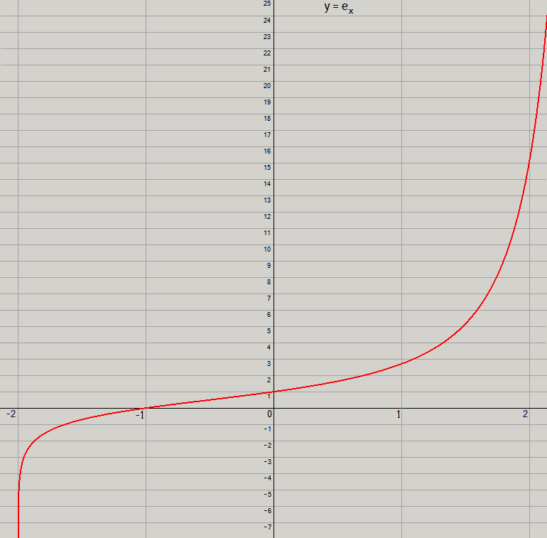
Features to note:

e_x is undefined for x ≤ –2. (It would involve the logarithm of a non-positive number.)

As x → –2⁺, e_x → –∞.

When x = –1, e_x = 0.

When x = 0, e_x = 1.

When x = 1, e_x = e = 2.71828 ... .

There is a point of inflection between –1 and 0. A graph is fairly straight near a point of inflexion; this graph is fairly straight throughout the entire interval from x = –1 to 0. Throughout that interval e_x differs from x + 1 by less than .01 .

Computer Program I
The following computer program can be modified for Visual Basic, FORTRAN and any other BASIC-like compiler.

This glossary translates the computer program functions into the mathematical functions of the above analysis when e(x) = exp(x) – 1.

Program	Analysis
DeLog(x)	A^’(x) = a(x) = 1 / Φ(x)
AsympDeLog(x)	1 / asymptotic power series for Φ(x)
eLog(x)	A(x)
eExpInteger(n, x)	e_n(x)
eExp(x)	A _{_– 1}(x)
ExpInteger(n, x)	exp_n(x)
ExpReal(s, x)	exp_s(x)

' The Fourth Operation I
'------------------------------------------------------------

Macro Precision         = Double              '15 or 16 significant digits
Macro expRealTol        = .00000001
Macro eExpTolNewton     = .00000001
Macro eLogDxMax         = .01
Macro CheckExit         = If exitflag Then Exit Function

Global e, em1, DeLog1 As Precision            'constants
Global exitflag, overflowflag As Long         'flags
'------------------------------------------------------------

%ht = 8             'cut off in power series, 8 max -- see Dim coef and Assign coef
Function AsympDeLog(x As Precision) As Precision
 Local i As Long
 Local sum As Precision
 Dim coef(8) As Static Precision              'make static so need assign only once

 CheckExit
 '                      0  1  2    3      4     5       6        7        8
 If coef(2) = 0 Then                          'first call?
  Array Assign coef() = 0, 0, 1/2, -1/12, 1/48, -1/180, 11/8640, -1/6720, -11/241920
 End If

 If     x < 0 Then
  Print "AsympDeLog: out of bounds" :exitflag = 1
  Exit Function
 ElseIf x = 0 Then
  Function = 0
  Exit Function
 End If

 ' sum starts as 0
 For i = 2 To %ht                'terms to x^5 give at least five decimal places if x < .05
  sum = sum + coef(i) * x^i
 Next

 Function = 1 / sum
End Function
'------------------------------------------------------------

%maxLogRep = 20
Function DeLog(x As Precision) As Precision
 Dim xx(%maxLogRep) As Precision
 Local d As Precision
 Local i, n As Long

 CheckExit

 If     x < 0 Then
  Print "DeLog: out of bounds" :exitflag = 1
  Exit Function
 ElseIf x = 0 Then
  Function = 0
  Exit Function
 End If

 ' n starts as 0
 xx(0) = x
 Do
  Incr n :If n > %maxLogRep Then Print "DeLog: failed" :exitflag = 1 :Exit Function
  xx(n) = Log(1 + xx(n - 1))
 Loop Until xx(n) < .1         'anything smaller doesn't affect output before 6 decimal places
                               'the smaller this, the larger %maxLogRep must be
 d = 1
 For i = 0 To n - 1
  d  = d * (1 + xx(i))
 Next

 Function = AsympDeLog(xx(n)) / d
End Function
'------------------------------------------------------------

Function eLog(ByVal x As Precision) As Precision   'integrate DeLog(t) from 1 to x
 Local cnt As Long                                 'use Romburg's Method of integration
 Local i, k, nmax As Long
 Local p As Long
 Local sum, h, dx As Precision

 CheckExit

 If x = 1 Then
  Function = 0
  Exit Function
 End If

 ' cnt starts as 0
 Do Until x < em1                      'get  x < e - 1,  eLog(x) < 1
  x = Log(1 + x)
  Incr cnt
 Loop
          
 dx = eLogDxMax                        'want nmax so  abs(x - 1) / 2^nmax  <=  dx
 Do Until dx < Abs(x - 1)              'is dx small enough?
  dx = dx / 2
 Loop
 nmax = 1 + Log2(Abs(x - 1)/dx)        'add one to ensure at least one
 Dim R(nmax,nmax) As Precision         'nmax does not exceed 7
                                       'now finished with dx, all we needed was nmax
 h = (x - 1) / 2
 R(0,0) = h * (DeLog1 + DeLog(x))      'DeLog1 = DeLog(1)

 For i = 1 To nmax
  h = (x - 1) / 2^i
  sum = 0
  For k = 1 To 2^(i-1)
   sum = sum + DeLog(1 + (2*k-1)*h)
  Next
  R(i,0) = R(i-1,0)/2 + h*sum
  p = 1
  For k = 1 To i
   p = p * 4
   R(i,k) = R(i,k-1) + (R(i,k-1) - R(i-1,k-1))/(p-1)      'p = 4^k
  Next
 Next

 Function = R(nmax,nmax) + cnt
End Function
'------------------------------------------------------------

Function eExpInteger(n As Long, ByVal x As Double) As Precision     'e sub n (1)
 Local i As Long

 CheckExit

 overflowflag = 0
 For i = 1 To n
  x = Exp(x) - 1
  If x = 1/0 Then overflowflag = 1 :Exit Function
 Next

 Function = x
End Function
'------------------------------------------------------------

%maxNewtonRep = 20
Function eExp(ByVal y As Precision) As Precision   'inverse of eLog, y >= 0
 Local x, xlast As Precision
 Local n, cnt As Long

 CheckExit

 cnt = 0                     'get fractional part of y
 Do Until y < 1
  Decr y
  Incr cnt
 Loop
 Do Until y >= 0
  Incr y
  Decr cnt
 Loop
 ' here  0 <= y < 1,  cnt = integral part of original y

 ' Newton-Raphson Method, it uses the derivative of eLog.
 ' n starts as 0
 x = 1
 Do
  xlast = x
  x = xlast + (y - eLog(xlast)) / DeLog(xlast)
  Incr n
  If n > %maxNewtonRep Then Print "eLog: hung" :exitflag = 1 :Exit Function
 Loop Until Abs(x - xlast) < eExpTolNewton
 Function = eExpInteger(cnt, (x + xlast) / 2)   'this will be 0 if overflow
End Function
'------------------------------------------------------------

' n must not exceed 3 or 4 (depends on x) to avoid overflow. And:
' If n = -1, x must > 0,  if n = -2, x must > 1,  if = -3, x must > e, ...
' in general if n < 0, x must > ExpInteger(-2 - n ,1)
Function ExpInteger(n As Long, ByVal x As Precision) As Precision
 Local i As Long

 CheckExit

 If n >= 0 Then
  For i = 1 To n
   x = Exp(x)
  Next
 Else
  For i = 1 To -n
   If x <= 0 Then
    Exit Function
   Else
    x = Log(x)
   End If
  Next
 End If

 Function = x
End Function
'------------------------------------------------------------

' This is the principal function.
Function ExpReal(ByVal s As Precision, ByVal x As Precision) As Precision
 Local p, y, z, zlast As Precision
 Local cnt, n As Long

 ' cnt starts as 0
 Do Until s < 1               'get fractional part of s
  Decr s
  Incr cnt
 Loop
 Do Until s >= 0
  Incr s
  Decr cnt
 Loop
 ' here  0 <= s < 1,  cnt = integral part of original s

 If s = 0 Then
  Function = ExpInteger(cnt, x)
  Exit Function
 End If

 If     x < 0 Then            'get 0 <= x < e
  x = Exp(x)
  Decr cnt
 ElseIf x >= e Then
  Do Until x < e
   x = Log(x)
   Incr cnt
  Loop
 End If
 
 ' n starts as 0,  z starts as 0
 Do
  zlast = z
  p = eLog(ExpInteger(n, x))
  y = eExp(p + s)
  If overflowflag Then        'this flag is set in eExpInteger, called by eExp
   z = 0
   Exit Do
  End If
  z = ExpInteger(-n, y)
  Incr n
 Loop Until Abs(z - zlast) < expRealTol Or z = 0 Or exitflag = 1

 If z = 0 Then
  Function = ExpInteger(cnt, zlast)
 Else
  Function = ExpInteger(cnt, z)
 End If
End Function
'===========================================================================

%list   = 1
%socket = 2
%graph  = 3
%which = %socket                    'one of the above

%xd = 180                           'used in the %graph case
%yf = 23
Function Main
 Local w, h, a, b As Long
 Local s As Precision

 Desktop Get Size To w, h            'set up console window
 Console Get Size To a, b
 Console Set Loc (w - a)\2, (h - b)\2
 Console Set Screen 120, 100

 e = Exp(1)                          'global constants
 em1 = e - 1
 DeLog1 = DeLog(1)
 
 Print Exp(-15)

 #If %which = %list '~~~~~~~~~~~~~~~~~~~~~~~~~~~~~~~~~~~~~~~~~~~~~~~~~~~~~~~

 Print "    "; " s", " e sub s"
 Print "    "; "----------------------"

 For s = -1 To 3.5 Step .125
  Print "    "; Format$(s,"* .000;-0.000"), Format$(ExpReal(s, 1)," #.00000")
 Next
 WaitKey$

 #ElseIf %which = %socket '~~~~~~~~~~~~~~~~~~~~~~~~~~~~~~~~~~~~~~~~~~~~~~~~~

 Local x As Precision

 Print " *** to exit, click X at upper right corner ***" :Print
 Print " This demonstration doesn't check that  s  and  x  are within"
 Print " bounds.  It will give a nonsensical result if in the course"
 Print " of the calculation the logarithm of a negative number would
 Print " have to be performed or a number is computed that is larger
 Print " than double precision can handle." :Print

 Do
  Input " Enter s operand:  "; s
  Input " Enter x socket:  "; x
  Print " exp sub"; s; "(";Format$(x,"#.0#####");")  =  "; Format$(ExpReal(s, x)," #.000000")
  Print
 Loop

 #Else  '%which = %graph '~~~~~~~~~~~~~~~~~~~~~~~~~~~~~~~~~~~~~~~~~~~~~~~~~~

 Local i, c As Long
 Local x, y As Precision
 Local winC As Dword

 Print "  *** to exit, click on this window and press Esc ***" :Print

 Graphic Window "", 100, 0, 768, 768 To winC        'set up graphic window
 Graphic Attach winC, 0
 Graphic Scale (-384,384+200) - (384,-384+200)
 Sleep 1

 For i = -9 To 29                                   'horizontal lines
  If i = 0 Then c = %Black Else c = &hA0A0A0
  Graphic Line (-384,i*%yf)-(384,i*%yf), c
 Next

 For i = -2 To 3                                    'vertical lines
  If i = 0 Then c = %Black Else c = &hA0A0A0
  Graphic Line (i*%xd,-384+200)-(i*%xd,384+200), c
 Next

 Graphic Width 2                                    'graph
 x = -2*%xd + .000001
 y = %yf*ExpReal(x/%xd, 1)
 Graphic Set Pixel (x, y)
 For x = -2*%xd + .000001 To 2.3*%xd
  y = %yf*ExpReal(x/%xd, 1)
  Graphic Line -(x,y), %Red
  If InStat And InKey$ = $Esc Then Exit Function
 Next

 WaitKey$
 #EndIf '~~~~~~~~~~~~~~~~~~~~~~~~~~~~~~~~~~~~~~~~~~~~~~~~~~~~~~~~~~~~~~~~~
End Function   
'------------------------------------------------------------

Another Path to the Same Destination
In finding the power series for Φ(x), the reciprocal of the derived Abel function for e^x – 1, we noted in a footnote that we could consider e_s(x) as a function of x with s as a parameter and showed that the power series for it begins:

e_s(x) ~ x + ½ s x² + ... as x → 0⁺

We briefly indicated how the rest of the coefficients, each a finite power series in s, could be determined. Then we chose to abandon that series, which is in two variables (even if one is called a parameter), and instead pursue a series for Φ(x), which is not only simpler, its analogy with x vis-à-vis log x suggests that it is more fundamental theoretically.

However we now resume the earlier line of inquiry. It offers a way to compute e_s(x) directly and a different way to determine the Abel function A(x) instead of integrating 1 / Φ(t) from 1 to x.

We need to compute more terms of the power series above. The rest of the coefficients can be determined by breaking e_s+1(x) two ways

e(e_s(x)) = e_s(e(x))

and plugging in the known power series for e(x) and what we know of the power series for e_s(x), then equating coefficients of like powers of x. As with the power series for Φ(x) a symbolic algebra calculator will help. We already have

c_₁ = 1
c_₂ = 1/2 s

Using the above procedure we find that the next three coefficients are

c_₃ = – 1/12 s + 1/4 s²
c_₄ = 1/48 s – 5/48 s² + 1/8 s³
c_₅ = – 1/180 s + 1/24 s² – 13/144 s³ + 1/16 s⁴

so that

e_s(x)

-as x → 0

x + 1/2 s x² + (– 1/12 s + 1/4 s²) x³ + (1/48 s – 5/48 s² + 1/8 s³) x⁴ + (– 1/180 s + 1/24 s² – 13/144 s³ + 1/16 s⁴) x⁵ + ...

As a check, try s = 1. In that case the coefficient of each power of x is the sum of the coefficients of the powers of s within it: 1, 1/2, 1/6, 1/24, 1/120, ..., which begins the Taylor expansion of e(x) = e^x – 1, as it should. (The series in that particular case converges for all x, which is not typical. I. N. Baker has shown that the function e_s(x) is analytic only when s is integral.)

Footnote
If we rearrange the series in powers of s:

e_s(x)

x + (1/2 x² – 1/12 x³ + 1/48 x⁴ – 1/180 x⁵ + ...) s + (1/4 x³ – 5/48 x⁴ + 1/24 x⁵ + ...) s² + (1/8 x⁴ – 13/144 x⁵ + ...) s³ + (1/16 x⁵ + ...) s⁴ + ...

(still as x goes to 0, not s) the coefficient of the first power of s appears to be the power series for Φ(x).

Note that s in the boxed series needn’t be near zero, it can be any number. As for x, in general only when it is near zero does the series give a good approximation. It can approach zero from above or below.

To use the series for a given x much different from zero, either raise or lower it by computing

e_k(x)

for k = 0, 1, 2, ... or k = 0, –1, –2, ..., depending on whether x is less than or greater than zero, until e_k(x) is near zero according to our chosen tolerance. Let n be that final k. Given s, we can use our power series to approximate

e_s(e_n(x))

Call it y. Then

e_s(x) ≈ e_–n(y)

Though the power series works for s any distance from zero it gives a little better approximation if s is between zero and one. We can add a whole number m, positive or negative, to s to get into that range, then after using the power series apply e_–m() to undo that operation. We can combine the two undoings, the one for x and the one for s, and just use n + m in the last formula above instead of n.

The following computer program implements this procedure. x near 0 is taken to mean |x| < .05, which makes the result accurate to about seven figures.

'  e sub s (x) directly using power series
'------------------------------------------------------------

Macro Precision = Double
Macro tol = .05

Global overflowflag As Long
'------------------------------------------------------------

Function eIterate(ByVal s As Precision, ByVal x As Precision) As Precision
 Local cnt, i As Long
 Local ss, sss As Precision
 Local y As Precision
 Local t As Precision

 cnt = Int(s)             'integer part of s
 s = s - cnt              'fractional part of s, it is now 0 <= s < 1

 Do Until x < tol         'drop x down to less than tol
  x = Log(x + 1)
  Incr cnt
 Loop
 Do Until x > -tol        'raise x up to greater than 0
  x = Exp(x) - 1
  Decr cnt
 Loop

 ss = s*s
 sss = ss*s
 y = x + _
     (s/2) * x^2 + _
     (-s/12 + ss/4) * x^3 + _
     (s/48 - 5*ss/48 + sss/8) * x^4 + _
     (-s/180 + ss/24 - 13*sss/144 + sss*s/16) * x^5

 If     cnt > 0 Then
  For i = 1 To cnt
   t = y
   y = Exp(y) - 1
   If y < t Then
    overflowflag = 1
    Exit Function
   End If
  Next
 ElseIf cnt < 0 Then
  For i = 1 To -cnt
   y = Log(y + 1)
  Next
 End If

 Function = y
End Function
'------------------------------------------------------------

Function PBMain
 Local w, h, a, b As Long
 Local s, x, y As Precision

 Desktop Get Size To w, h            'set up console window
 Console Get Size To a, b
 Console Set Loc (w - a)\2, (h - b)\2
 Console Set Screen 120, 100

 Print " *** to exit, click X at upper right corner ***" :Print
 Print

 Do
  Input " Enter s parameter:  "; s
  Input " Enter x variable:   "; x
  overflowflag = 0
  y = eIterate(s, x)
  If overflowflag Then
   Print "   overflow"
  Else
   Print " e sub"; s; "(";x;")  =  "; Format$(y," #.00000000000000")
  End If
  Print
 Loop

 WaitKey$
End Function
'-----------------------------------------------------------------

In the section “To Proceed” we computed the Abel function A(x) for e(x) = e^x – 1 on the way to computing e_s(x). In the above we used a power series for e_s(x) to compute e_s(x) directly.

The e_s(x) power series can also be used to compute A(x). Recall that the Abel function for e(x) is a sort of “functional logarithm” or “logarithm of iteration” that measures the amount of iteration of e(x) in a variable. Precisely (see the section “Facts About Functions” above and apply it to f(x) = e(x) = e^x – 1) these two equations are equivalent:

y = e_s(x)
A(y) = A(x) + s

Now suppose we have the power series beginning this section. Given x ≥ 1, we can use it to compute A(x) as follows.

We already know A(1) = 0. Let x = x₀ > 1. Then compute

x_k = e_–k(x)

for k = 0, 1, 2, ... (here k is just a subscript), making k large enough so that x_k is near zero according to our chosen tolerance. Let n equal that last k. Let

u_n = e_–n(1)

It will be even nearer zero.

Now consider the difference

A(x_n) – A(u_n)

It is

A(e_–n(x)) – A(e_–n(1))

( A(x) – n ) – ( A(1) – n )

The n’s cancel. Since A(1) = 0 we have

A(x_n) – A(u_n) = A(x)

independent of n.

Recall that our goal is to find A(x) given x. Let s = A(x). The following are equivalent:

A(x_n) – A(u_n) = s

A(x_n) = s + A(u_n)

x_n = e_s(u_n)

Since u_n is near zero we can use our power series to approximate e_s(u_n); the larger n is the better the approximation. We know e_–n(x) and e_–n(1), so we can solve the last equation for s using our power series for e_s(x). Rapheson’s Method (a.ka. the Secant Method) could be used.

We need compute A(x) only for x less than e – 1, that is, x in the range [1, e – 1). From such values of A(x) we can determine A(x) for greater x by using e_–1() and the formula for A():

A(x) = A(e_–k(x)) + k

where the whole number k is just large enough so that e_–k(x) <= 1. To find A(x) for x in the range (0, 1] use A(x) = A(e(x)) – 1.

Footnote
The last part of this section is a simplified account of the method given in Morris & Szekeres’s addendum to the first reference cited in our “Introduction.” Our lemmas #0, #1, and #2 allowed us to prove that the second-order coefficient in the power series above is _½ s, patching a serious gap in their argument.

Morris & Szekeres go out of the way to, in a manner of speaking, bring s near zero as well as x and 1 but that is unnecessary if each coefficient, a finite series in s, is determined in full instead of truncating them. (Truncating these finite series probably contributed to the accumulation error they mention.)

Computer Program II
We can use the computer code at the end of the first part of the previous section “Another Path” – which iterates e(x) – along with the “wash out” procedure described at the beginning of “The Original Problem” – which turns iterates of e(x) into iterates of exp(x) – to find iterates of exp(x), that is, to compute the fourth operation.

The resulting computer program is much simpler than “Computer Program I.” Here is a glossary translating the computer program functions into the mathematical functions we used in the first part of the previous section.

Program	Analysis
eExp(s, x)	e _s(x)
ExpInteger(n, x)	exp_n(x)
ExpReal(s, x)	exp_s(x)

' The Fourth Operation II
'------------------------------------------------------------

Macro Precision   = Double
Macro expRealTol  = .0000001
Macro tol         = .01

Global e As Precision            'constant
Global overflowflag As Long      'flag
'------------------------------------------------------------

Function eExp(ByVal s As Precision, ByVal x As Precision) As Precision
 Local cnt, i As Long
 Local ss, sss As Precision
 Local y As Precision

' s has already been put in range by caller,  0 <= s < 1

 Do Until x <  tol        'drop x down to less than tol
  x = Log(x + 1)
  Incr cnt
 Loop                     'or else
 Do Until x > -tol        'raise x up to greater than 0
  x = Exp(x) - 1
  Decr cnt
 Loop

 ss = s*s                 's^2
 sss = ss*s               's^3
 y = x + _
     (s/2) * x^2 + _
     (-s/12 + ss/4) * x^3 + _
     (s/48 - 5*ss/48 + sss/8) * x^4 + _
     (-s/180 + ss/24 - 13*sss/144 + sss*s/16) * x^5

 If     cnt > 0 Then
  For i = 1 To cnt
   y = Exp(y) - 1
  Next
 ElseIf cnt < 0 Then
  For i = 1 To -cnt
   y = Log(y + 1)
  Next
 End If

 Function = y
End Function
'------------------------------------------------------------

Function ExpInteger(ByVal n As Long, ByVal x As Precision) As Precision
 Local i As Long

 If n >= 0 Then
  For i = 1 To n
   x = Exp(x)
  Next
 Else
  For i = 1 To -n
   If x <= 0 Then
    overflowflag = 2
    Exit Function
   End If
   x = Log(x)
  Next
 End If

 Function = x
End Function
'------------------------------------------------------------

' This is the main function.
Function ExpReal(ByVal s As Precision, ByVal x As Precision) As Precision
 Local y, v, lasty As Precision
 Local cnt, n As Long

 cnt = Int(s)                 'whole part of s
 s = s - cnt                  'fractional part of s, it is now 0 <= s < 1
 ' here  0 <= s < 1,  cnt = integral part of original s

 If s = 0 Then
  overflowflag = 0
  Function = ExpInteger(cnt, x)
  Exit Function
 End If

 If     x < 0 Then            'get 0 <= x < e
  x = Exp(x)
  Decr cnt
 ElseIf x >= e Then
  Do Until x < e
   x = Log(x)
   Incr cnt
  Loop
 End If

 y = eExp(s, x)               'n = 0
 lasty = y
 n = 1
 Do
  overflowflag = 0
  v = expInteger(-n, (eExp(s, expInteger(n, x))))
  If overflowflag Then Exit Do    'use last y
  y = v
  If Abs(y - lasty) < expRealTol Then Exit Do    'Cauchy convergence
  lasty = y
  Incr n
 Loop

 Function = expInteger(cnt, y)
End Function
'===========================================================================

%list   = 1
%socket = 2
%graph  = 3
%which = %socket                    'one of the above

%xd = 180                           'used in the %graph case
%yf = 23
Function Main
 Local w, h, a, b As Long
 Local s As Precision

 Desktop Get Size To w, h           'set up console window
 Console Get Size To a, b
 Console Set Loc (w - a)\2, (h - b)\2
 Console Set Screen 120, 100

 e = Exp(1)                         'global constant

 #If %which = %list '~~~~~~~~~~~~~~~~~~~~~~~~~~~~~~~~~~~~~~~~~~~~~~~~~~~~~~~

 Print "    "; " s", " e sub s"
 Print "    "; "----------------------"

 For s = -1 To 3.5 Step .125
  Print "    "; Format$(s,"* .000;-0.000"), Format$(ExpReal(s, 1)," #.00000")
 Next
 WaitKey$

 #ElseIf %which = %socket '~~~~~~~~~~~~~~~~~~~~~~~~~~~~~~~~~~~~~~~~~~~~~~~~~

 Local x As Precision

 Print " *** to exit, click X at upper right corner ***" :Print
 Print " This demonstration doesn't check that  s  and  x  are within"
 Print " bounds.  It will give a nonsensical result if in the course"
 Print " of the calculation the logarithm of a negative number would
 Print " have to be performed or a number is computed that is larger
 Print " than double precision can handle." :Print

 Do
  Input " Enter s operand:  "; s
  Input " Enter x socket:  "; x
  Print " exp sub"; s; "(";Format$(x,"#.0#####");")  =  "; Format$(ExpReal(s, x)," #.000000")
  Print
 Loop

 #Else  '%which = %graph '~~~~~~~~~~~~~~~~~~~~~~~~~~~~~~~~~~~~~~~~~~~~~~~~~~

 Local i, c As Long
 Local x, y As Precision
 Local winC As Dword

 Print "  *** to exit, click on this window and press Esc ***" :Print

 Graphic Window "", 100, 0, 768, 768 To winC        'set up graphic window
 Graphic Attach winC, 0
 Graphic Scale (-384,384+200) - (384,-384+200)
 Sleep 1

 For i = -9 To 29                                   'horizontal lines
  If i = 0 Then c = %Black Else c = &hA0A0A0
  Graphic Line (-384,i*%yf)-(384,i*%yf), c
 Next

 For i = -2 To 3                                    'vertical lines
  If i = 0 Then c = %Black Else c = &hA0A0A0
  Graphic Line (i*%xd,-384+200)-(i*%xd,384+200), c
 Next

 Graphic Width 2                                    'graph
 x = -2*%xd + .000001
 y = %yf*ExpReal(x/%xd, 1)
 Graphic Set Pixel (x, y)
 For x = -2*%xd + .000001 To 2.3*%xd
  y = %yf*ExpReal(x/%xd, 1)
  Graphic Line -(x,y), %Red
  If InStat And InKey$ = $Esc Then Exit Function
 Next

 WaitKey$
 #EndIf '~~~~~~~~~~~~~~~~~~~~~~~~~~~~~~~~~~~~~~~~~~~~~~~~~~~~~~~~~~~~~~~~~
End Function
'-----------------------------------------------------------------

Is it Unique?
The question of uniqueness bedevils attempts to define the fourth operation. We first showed that exp(x) – 1 has a continuum of iterates e_s(x) and it is unique. Then we defined exp_s(x) in terms of e_s(x); however we did not prove it is unique.

Using a different approach Szekeres showed “by partly intuitive arguments” that the Abel function of e(x), since that function is well-behaved in a certain way near zero (and likewise well-behaved at infinity), merits being used as a comparison function that determines a unique Abel function for any reasonable function. What recommends his idea of well-behaved is hard to follow.

Bases Other Than e
What if we wanted to know 2_½ instead of e_½? And in general b_s for other bases? We can again use the “socket” idea and functional analysis: let f (x) = b^x and find its functional iterates. Note that to ensure f (x) is real and continuous b must exceed zero.

We will try to develop functional iterates around a fixed point as we did before when b was e. Now in that case f (x) had no fixed point so we resorted to the artifice of first considering f (x) minus one. However for general b, in some cases we have a fixed point to begin with, in fact perhaps two; the number depends on what range of the real line b is in. We can determine them by examining the intersection of the graph of y = b^x with the graph of y = x. The ranges break at zero, one, and the e^th root of e.

	range of b	# of fixed points of f (x) = b^x
1.	0 < b ≤ 1	1 (the graph crosses y = x)
2.	1 < b < e^1/e	2 (it crosses y = x over and back)
3.	b = e^1/e	1 (it is tangent)
4.	b > e^1/e	0 (it is separate)

If the first case, where f (x) has exactly one fixed point, we can use the fact (pointed out in a footnote after the proof of Lemma #1 above) that for any function f (x) having a fixed point at x = a,

f _s ^’(a) = (f ^’(a)) ^s

That gives an extra term of our power series so we can find the other terms directly.

The second case is a problem. We could do at each point what was suggested in the first case just considered but that would result in two different functional iterates of the given function. Another problem with having more than one fixed point is that then there could be no single Abel’s function. Recall that the Abel function A(x) must be defined for x > 0 and

A(e(x)) = A(x) + 1

If for example f (x) = 2^x – 1, which has a fixed point at zero and at one, then A(x) could not be defined at x = 1. The Abel function will always be singular at a fixed point. We will return to the second case in a moment.

The third case, where f ^’(a) = 1, can be solved with the methods we used for f (x) = e^x – 1, which has exactly one fixed point, at zero, and f ^’(0) = 1. The details will be given when we examine the fourth case of which the third is a limiting case: as b approaches e^1/e from below, the graph y = f (x) approaches touching the graph of y = x.

The fourth case, like the second, is a problem. We will try to solve it as well as the second by translating f (x) = b^x so it just touches y = x, as we did with f (x) = e^x.

Note that in the first and third cases no translation artifice is necessary, so the resulting fractional iterates are demonstrably unique, just as those of e^x – 1 were.

We will use the same labels for the various functions as before. We need to define e(x) having a unique fixed point whose percentage difference with b^x goes to zero (that is, their ratio goes to one) as x goes to infinity.

To accomplish that we shall translate the graph of y = b^x vertically by an amount that makes it tangent to y = x. In general, unlike the case when b = e, the tangent point will not be at the origin. To simplify expressions, in what follows let

r = log b

where as usual log is the natural logarithm. Note that

b^x = e^rx

and when b = e, r = 1.

Setting the derivative of y = b^x to 1 (the slope of y = x) and solving for x gives x = – (log r) / r. Again to simplify future expressions let

u = – (log r) / r

Note that

b^u = 1/r

So the point (u, 1/r) on the graph of y = b^x is where the slope is 1. Thus if we translate by – (1/r – u), letting

e(x) = b^x – (1/r – u)

then e(u) = u and that is the only fixed point. The derivative is

e^’(x) = r b^x

In the special case where the base b = e^1/e, which is 1.44466786..., we have r = 1/e, u = e so that 1/r – u = 0, and no translation is necessary, y = b^x itself has exactly one fixed point, at x = e. (This is the third case above, where the graph is tangent to that of y = x.) In this case, to repeat, the continuous iterates are demonstrably unique.

Let A(x) be an Abel function for the new e(x)

A(e(x)) = A(x) + 1

and let

a(x) = A^’(x)

be the corresponding derived Abel function. Schröder’s equation for the new e(x) is

Φ(e(x)) = r b^x Φ(x)

As before we want to determine the Taylor series of Φ(x) but this time at x = u.

Φ(x) ~ c_₀ + c_₁ (x – u) + c_₂ (x – u)² + c_₃ (x – u)³ + ... as x → u⁺

Taking the first and second derivatives of each side of Schröder’s equation and evaluating at u we can, as before, eventually conclude that Φ^’(u) = 0 and Φ^’’(u) = 0, so that both c₀ and c₁ in the Taylor expansion are 0.

Φ(x) ~ c_₂ (x – u)² + c_₃ (x – u)³ + ... as x → u⁺

Again we need another coefficient and turn to finding the Taylor expansion of e_s(x), first in powers of (x – u) and then in powers of s.

As before we take the first derivative with respect to x of each side of e_s(x) = e(e_s–1(x)) and evaluate at u to eventually obtain

e_s^’(u) = e_s–1^’(u)

and so

e_s^’(u) = e_t^’(u)

where t is the fractional part of s. Thus as before e_s^’(u) = 1 when s is a whole number and the same proof as before shows this is true for all real s.

Taking the derivative with respect to x again and evaluating at x = u eventually leads to

e_s^’’(u) = r + e_s–1^’’(u)

so that

e_s^’’(u) = n r + e_t^’’(u)

where n and t are the integral and fractional parts of s respectively. Thus when s is a whole number e_s^’’(u) = s r and a similar proof as before shows this holds for all real s.

Thus the Taylor expansion begins:

e_s(x) ~ (x – u) + 1/2 s r (x – u)² + ... as x → u

Footnote
Determining the Taylor expansion of e_s(x) viewed as a function of s goes exactly as before and we have

e_s(x) ~ x + Φ(x) s + c_₂ s² + c_₃ s³ + ... as s → 0

We are trying to find Φ(x) . We proved that its Taylor expansion begins

Φ(x) ~ c_₂ (x – u) ² + c_₃ (x – u) ³ + c_₄ (x – u) ⁴ + ... as x → u⁺

and if, as before, we know just c_₂ we can determine the others. An argument similar to the one before shows that the second-order coefficient in the power expansion of Φ(x) is ½ r.

Thus we have

Φ(x) = 1/2 r (x – u) ² + c_₃ (x – u) ³ + c_₄ (x – u) ⁴ + ... as x → u⁺

Now we use Schröder’s equation to determine the other coefficients. Schröder’s equation is

Φ(e(x)) = r b^x Φ(x)

Φ(e^rx – 1/r + u) = r e^r x Φ(x)

Substituting in the power series as we did before when b = e we can deduce that

c₃ = (1/48 u² r⁴ – 1/6 u r³ + 7/24 r² – 1/3 r³)
/ (27/8 r² – 2 r – 7/8 +1/24 u³ r³ + 1/2 u² r² + 3/2 u r)

and succeeding coefficients can be computed likewise. If b = e then r = 1 and u = 0; and c₃ reduces to – 1/12 and c₄ to 1/48, the values we found before. When b = 2, c₃ = – .053891092257005... and c₄ = .00280571012920368... .

Repeated application of

e_-1(x) = logarithm to base b of (x– u + 1/r) = (1/r) log (x – u + 1/r)

will reduce any x > u to as close to u as desired. Given x₀ > u, let x_i = e_-i(x₀), then using Schröder’s equation as before we can eventually conclude

Φ(x₀) = rⁿ (x₀ + v) (x₁ + v) ... (x_n-1 + v) Φ(x_n)

where v = 1/r – u. Since u might exceed zero we also need to consider the case x₀ < u. Repeated application of e(x) will increase x₀ to as close to u as desired. Let x_i = e_i(x₀), then

Φ(x₀) = Φ(x_n) / rⁿ(x₁ + v)(x₂ + v) ... (x_n + v)

Thus we have Φ(x) and consequently A(x) and the continuous iterates of e(x). We can get from continuous iterates of e(x) to those of b^x by the same method as before except that exp and log are replaced with exp and log to the base b.

In the special case b = e^1/e this last step is unnecessary because then e(x) = b^x. In that case, the third case above, to repeat, the iterates are unique. When 0 < b ≤ 1 there is also exactly one fixed point and again the continuous iterates are unique. Furthermore, the graph of y = b^x is not tangent to the graph of y = x so they are much easier to compute.

Review and a Glance at the Complex Plane
We sought to define e raised to itself s times where s can be fractional. We added a sort of “socket” variable to turn the problem into defining continuous iterates of the function exp(x).

Since finding a unique continuous iterate of a function that has no fixed point, such as exp(x), is difficult, instead we considered the function exp(x) – 1, which has exactly one fixed point. Following George Szekeres (1911 – 2005) and patching up gaps in his work, we found by an intricate argument assuming only smoothness, a unique solution for the continuous iterates of that function.

Then we used it to find a solution for the continuous iterates of exp(x). However its uniqueness is a problem.

So far all we have used is real analysis. Another way to get around the fact that exp(x) has no fixed point is to go into the complex plane to find one, that is, consider exp(z) where z varies over the complex numbers. The trouble is that exp(z) has more than one fixed point, indeed an infinite number, and that leads to singularities and non-uniqueness. There are ways of dealing with the singularities but to get uniqueness requires further conditions. In any case Hellmuth Kneser (1898 – 1973) used one fixed point to construct an analytic solution, and later other people improved on his work. As for numerical results, Kneser’s solution differs from the one obtained by the Φ(x) approach. For example, e_½ is 1.64515… per our calculation whereas it is 1.64635… per Kneser’s.

There are many Kneser’s iterations, one for each fixed point. Ultimately the choice is arbitrary – one fixed point is like another – so Kneser’s primary iteration is not unique. Conditions can be posited to make a particular fixed point special but are they reasonable conditions?

At any rate, even if we failed with exp(x), the continuous iteration of e(x) = exp(x) – 1, solved here for the first time without arbitrary assumptions, is interesting in its own right.

Footnote
Szekeres was interested in continuously iterating e(x) in order to interpolate G. H. Hardy’s logarithmico-exponential scale. A(x), its Abel function, grows more slowly than any finite iteration of log(x) and the inverse grows more rapidly than any finite iteration of exp(x), thus these two functions are respectively below and above Hardy’s scale. (Note that Szekeres more than once mistakenly refers to a(x), the derived Abel function, when he means A(x).)

A Zero^th Operation?
In the introduction we took addition to be the first and basic operation. Some people have tried to define a zero’th operation before addition, called “succession.” It is a unary operation that increments its operand. Then iterating it on A, B times, would add B to A.

There are several problems with this zero’th operation. It is not a binary operation like the other operations. And since incrementing is a particular case of addition, it isn’t as different as a new operation should be.

A third problem involves this curious sequence:

2 + 2 = 4
2 · 2 = 4
2^² = 4

which continues ad infinitum. Letting [n] denote the n^th operation,

2 [n] 2 = 4

for all n. That is, for all n ≥ 1. Each operation “collapses” to the one below until you get to 2 + 2 at the bottom. You can also see that it is true by considering the recursive formula given in the introductory section of this article. We’ve seen that it is true when n = 1. For n > 1:

A [n] (B + 1) = A [n – 1] ( A [n] B )

Plug in A = 2 and B = 1 so we have 2 operated on by 2 in the left expression:

2 [n] 2 = 2 [n – 1] ( 2 [n] 1 )

For n > 1 the right operand on the right equals 2, and we have

2 [n] 2 = 2 [n – 1] 2

We could make, rather artificially, succession a binary operation by having it increment one of the two operands and ignore the other (for the recursion formula given in the introduction to work it would have to increment the second operand), but then the “2 on 2 theorem” would fail:

2 [0] 2 = 2 + 1 = 3

The 2 on 2 theorem is a nice little theorem. That it doesn’t hold for [0] suggests that [0] is illegitimate.

For all these reasons, the bottom operation should be addition, [1], rather than succession.

There is no zero’th operation.

While we’re on the subject of the specialness of addition, note that its “unit” – the number for the second operand that doesn’t affect the first – is zero. For any A:

A + 0 = A

Whereas with the operations beyond addition, n > 1, the unit is one:

A [n] 1 = A

It is also interesting to note that for operations beyond multiplication, n > 2:

A [n] 0 = 1

which follows from the recursion formula given in the introduction. When n = 1 or 2 (addition or multiplication) the result is A or 0 respectively. (Not only are addition and multiplication different from each other, this change after multiplication suggests that the two are fundamentally different operations from exponentiation when we try to make them the beginning of a series, a subject we will return to in the last section.)

Other Terminology and Notation
The fourth operation is known by various names: tetration, super-exponentiation, hyperpowers, power towers.

Instead of the subscript notation e_s some authors use the pre-superscript notation ^se (Hans Maurer (1868 – 1945) used it in a paper of 1901). Other notations, which generalize to operations of other order, are H₄(e, s), and Donald Knuth’s arrow notation e ↑↑ s (the number of arrows, two less than what you would expect, is confusing).

Given X = b_p the inverse operation giving b has been called the super-root, denoted by srt _p X. The inverse operation giving p has been called the super-logarithm, denoted by slog _{_b} X. (Rarely, “tetra” has been used instead of “super” while retaining the slog and srt notation.)

Afterword
A case could be made that there is no sequence of operations as presented in our introduction, that there are only two binary operations, addition and multiplication; that exponentiation is not a binary operation but a unary one (the exponent) with a parameter (the base). As a unary operation its purpose is to turn addition into multiplication; it is a go-between for two binary operations but not a binary operation itself.

Exponentiation cannot be a true binary operation because it cannot be defined when the base is negative and the exponent varies continuously.

Even restricted to positive numbers, because of the non-associatively of exponentiation it cannot be a group operation.

Another reason exponentiation stands out from addition and multiplication is that it has no geometric construction that is continuous in the exponent. Addition can be thought of as laying two line segments end to end in a straight line, multiplication as the area indicated when line segments are joined perpendicularly. We run into a problem with exponentiation. X, X squared, X cubed, etc. make sense geometrically – a line segment, square, cube, and so forth in higher dimensions – but there is no continuum of dimensions to make sense of X raised to a fraction. What, for example, is between a square and a cube? (The fractional and continuous geometries of Menger, Birkoff, and von Neumann are no help because their dimensions range between zero and one, and they are projective geometries rather than Euclidean.)

A further difference – among all three of addition, multiplication, and exponentiation – becomes apparent when using the operations to solve practical problems. In practice many numbers are not pure numbers but quantities, that is, they measure something in a certain unit such as meters or kilograms. We will say a pure number has the “null unit” so that all numbers have units. When adding two numbers both must be in the same unit. As the saying goes, “You can’t add apples and oranges.” When multiplying there is no such restriction, each number can have any unit. When neither number is pure the result is in a new unit. For example, two meters times three meters is six square meters, two watts times three hours is six watt-hours.

Multiplication can be considered repeated addition only when one of the numbers – the number measuring the repetition – is pure. Adding five apples to itself three times makes 15 apples, but using three apples or three oranges as a count for adding makes no sense.

With exponentiation, the exponent must be pure. (An exponent might be an expression involving quantities but when evaluated the units must cancel.) In physics, if the exponent can vary continuously the base must be pure as well. In general there is no exponentiation of quantities.

With what we have called the fourth operation, both base and “super-exponent” must be pure. (We could except the trivial cases where the super-exponent is 0 or 1, resulting in 1 or the base respectively.) This suggests that this so-called operation could have no practical application beyond generating large pure numbers, and then only whole number iterates would be needed.

Thus it would seem we have gone on a fool’s errand, though an interesting one. Not only is there no fourth operation, there is not even a third operation. Exponentiation, to repeat, should not be viewed as a third binary operation or as any kind of binary operation. It is a unary operation on pure numbers, or rather a continuum of unary operations parameterized by a base. It is a bridge between the two elementary operations on numbers stripped of their units that converts addition to multiplication and whose inverse converts multiplication to addition.

Simple fractional (rational) exponents are useful in physics, in which sase the denominator indicates a root. In mathematics, when trying to describe the growth of a function as a variable goes to infinity, a real (even transcendental) exponent can be useful.