<< Algorithms
Random Yet Smooth Motion
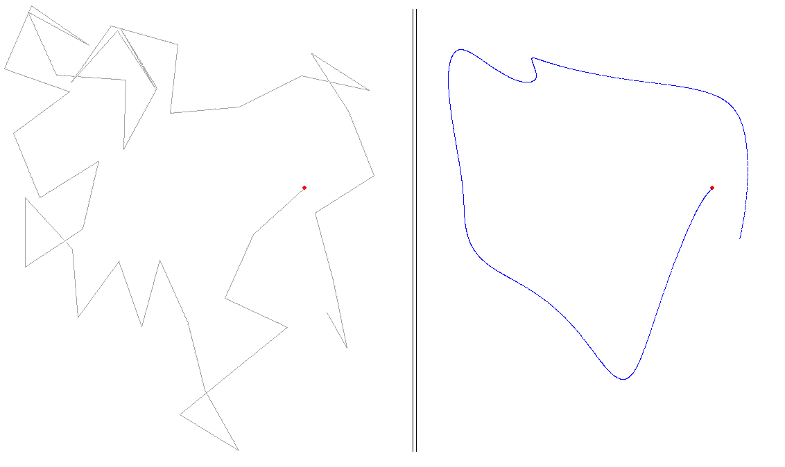
Imagine a point moving in a plane. We seek a motion that is both random and at the same time smooth. Those characteristics might seem to be at odds with one another. If the motion is smooth then given a point in time, a short time later it would be near by, it would be going in nearly the same direction as it had been going. The point’s immediate future position would be approximately predictable.
The key to the solution is to realize that we can start with another path that isn’t computed “as we go” but computed ahead of time into the future. We can make this path as random as we want, even if not smooth, then smooth it later. By considering a time interval only partly into the future, we can compute the path as we go along. Details follow.
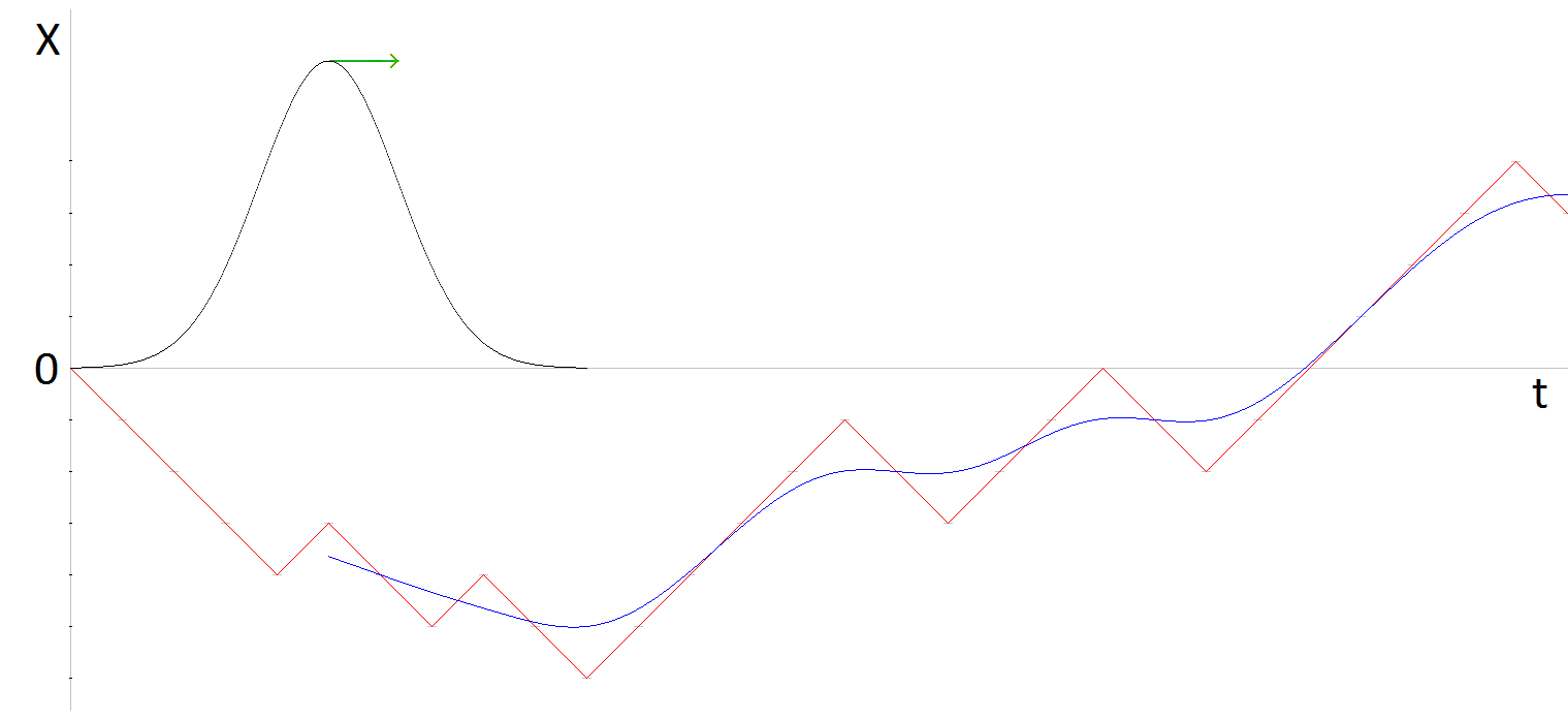
First consider a random walk on the line, placed vertically so its trajectory can be graphed with time as the horizontal axis. Each step of the point is taken up or down at random. In the following diagram the graph of the random walk, X(t), is colored red. Then take the running average over a number of steps, say 10. Better, take the weighted average using a bell-shaped function. In the diagram the graph of the resulting smooth motion X̅(t) is colored blue. In signal jargon, the running average is a low pass filter. Mathematically the running average is the convolution of the random-walk with the weight function.

Now consider a random walk in the plane and do such a convolution on each dimension separately. Start with the “drunkard’s walk”: choose a random direction and move one step in that direction, then repeat. Now consider the projection of that motion onto the X and Y axes, so you have two functions of time X(t), Y(t). Consider each function separately. The graph is angular and bumpy. After the walk has progressed for a certain number of steps – say 10 – start taking the running average weighted by a bell shaped curve whose width covers 10 steps (in other words, convolve each of X(t) and Y(t) with a bell shaped curve 10 steps wide). That smoothes the two functions. Then combine them again to trace out a random but smooth motion X̅(t), Y̅(t).
The moving point might slow, come to a stop, reverse direction and accelerate. In that case, though the path is not smooth at the turning point the motion is. The qualification smooth applied to the motion of a point means that its velocity varies continuously.

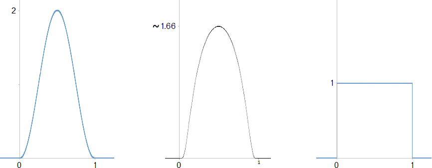
A suitable weight function is positive within the interval 0 to 1, zero outside it, and its integral is one. In use the interval can be scaled to cover the number of steps required. Example weight functions:

The first example is the cosine function in the interval –π to π, suitably scaled and shifted:
1 + cos 2π (x – ½)
for x between 0 and 1.
The second example is
A e 1 / ( (2x – 1) 2 – 1)
where A is about 4.5 so the integral from 0 to 1 is 1. When x = ½ this function is about 1.66 so its graph is a bit fatter than that of the first weight function above. By replacing the exponent 2 with a larger, even, exponent, you get a still fatter graph.
The third is the “rectangular step function.” It gives the uniformly weighted average.
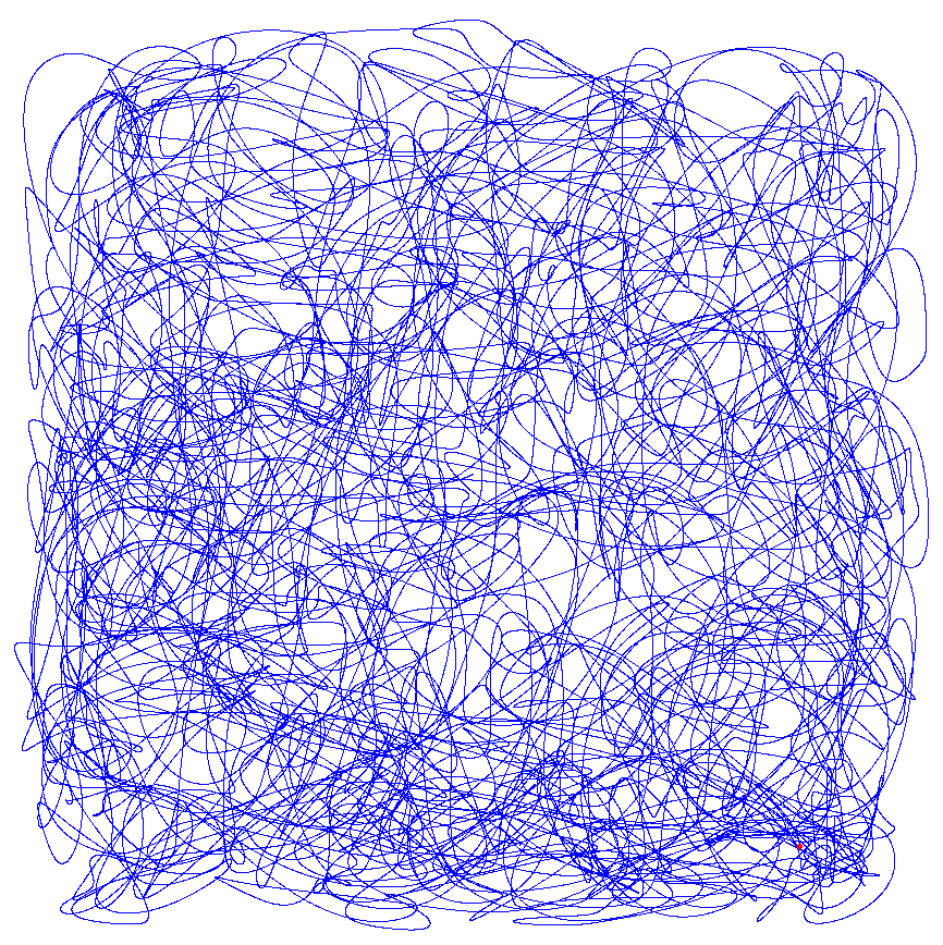
It turns out that any more or less bell shaped curve will do for the weight function. Even the rectangular function, in other words an ordinary average instead of a weighted one, makes little difference in the general look of the resulting curve. The program below uses the first weight function graphed above.
A novel feature of the algorithm, found among the papers of M. Ralston, presented in the program below is that the smooth trajectory is computed as the random walk progresses. After computing an initial ‘F’ steps, the smooth trajectory is prolonged one step at a time.
Because we choose a random direction for each step of the random walk and then project onto X and Y, the projected length of the step varies, between zero and the step length in the plane. The average projected length is 2 / π times the planar step length.
In the program below, the moving point is prevented from wandering outside the graphic window as follows. If a random step would go outside the window, another random step is tried until it doesn’t. (Without this restriction, in dimensions one or two a random walk eventually returns arbitrarily close to its starting point, and every other point in the plane. In three or higher dimensions it might wander off never to return.)
The source code can be modified for Visual Basic, FORTRAN, or any other BASIC-like compiler. An executable (for Windows computers) with an added interface that allows you to change various parameters without re-compiling, can be downloaded from here.
If we choose for the weight function the rectangular function, that is, we take the simple running average, then bumpf() below is identically one. In that case its declaration, preliminary computation, and all “* bumpf(...)” can be removed.
' Defining constants ...
' F is the most important. STEPLEN should be smaller the larger F is, to
' better fit in the window.  M should be about STEPLEN for a solid line.
Const F = 3                           'number of steps to average over
Const STEPLEN = 150                   'step length
Const M = 150                         'number of points in one step of the random walk
' larger F, fewer tight loops;
' larger STEPLEN, magnify drawing (also points of trajectory further apart);
' larger M, points of trajectory closer together;

' Derived constant
Const N = M * F                       'total number of points to average over

' Speed constant
Const DELAY = 2                       'the larger this is the slower the random walk

' Compiler switch
#Const showsteps = -1                 'show the random walk or not
'-------------------------------------------------------------------------------------

Function PBMain
 Local i, j, k As Long                'indices for the most part
 Local winC As Dword                  'handle of graphic window
 Local xbrown0, ybrown0 As Single     'beginning of brownian step
 Local xbrown1, ybrown1 As Single     'end
 Local limit As Long                  'half screen height
 Local x, y As Single                 'current point
 Local dx, dy As Single               'change in direction of step
 Local th As Single                   'angle of a step
 Local pd As Single                   'pi doubled
 Dim xline(M - 1) As Single, yline(M - 1) As Single
 Dim xbrown(N - 1) As Single, ybrown(N - 1) As Single
 Dim bumpf(N - 1) As Single           'weight function
'-------------------------------------------------------------------------

 ' Set up graphic window, a square window that fills the screen vertically
 Desktop Get Client To i, j             'get computer’s screen size, horizontal & vertical
 Console Set Loc 0, j + 1               'hide console window
 Graphic Window "", (i - j) / 2,0, j,j To winC    'create graphic window
 Graphic Attach winC, 0, ReDraw         'choose it, specify drawing not shown until ReDraw
 limit = j / 2                          'half the window height
 Graphic Scale (-limit, limit) - (limit, -limit)  '(0, 0) at center of graphic window

 ' Instructions to user
 Graphic Set Focus
 Sleep 10
 Graphic Font "calibri", 15, 0
 Graphic Print
 Graphic Print "       To start a new path, press Spacebar."
 Graphic Print
 Graphic Print "       Now press Spacebar, or Esc to quit."
 Graphic ReDraw
 Do                                     'place and keep console in focus
  Console Set Focus
  Sleep 100
 Loop Until InStat
 If WaitKey$ = $Esc Then Exit Function  'wait for a key to be pressed

 Randomize Timer                        'random seed for Rnd
'-------------------------------------------------------------------------

 pd =  8 * Atn(1)                       'compute 2 * pi

 ' Pre-compute the weight function.  Note that  (i - N / 2) / N   =   i / N - 1/2.
 ' Because the integral from 0 to 1 of the function  1 + Cos 2(pi)(x - 1/2)
 ' equals 1, the sum of  bumpf(0 to N - 1)  equals, to many decimal places, N.
 ' In use, after multiplying by the weight function and summing, divide by N.
 For i = 0 To N - 1
  bumpf(i) =  1 + Cos(pd * (i - N / 2) / N)
 Next

 Do                                     'new path

  xbrown0 = 0 :ybrown0 = 0
  Reset xbrown(), ybrown()
  Graphic Clear

  Graphic Ellipse (-2, 2) - (3, -3), %Red, %Red           'draw starting dot
  Graphic ReDraw
  Sleep 200                                               'slight pause

  Do                                                      'F random walk steps

   Do
    th = pd * Rnd                                         'between 0 and two pi
    dx = Cos(th) * STEPLEN                                'random direction,
    dy = Sin(th) * STEPLEN                                'keep trying until within window
    xbrown1 = xbrown0 + dx
    ybrown1 = ybrown0 + dy
   Loop Until xbrown1 > -limit And xbrown1 < limit And ybrown1 > -limit And ybrown1 < limit

   For j = 0 To M – 1                                     'step from brown0 to brown1
    xline(j) = xbrown0 + dx * j / M
    yline(j) = ybrown0 + dy * j / M
   Next

   #If showsteps Then                                     'show random walk in light gray
   Graphic Line (xbrown0, ybrown0) - (xbrown1, ybrown1), &Ha0a0a0
   Graphic ReDraw
   #End If

   If DELAY Then Sleep DELAY

   xbrown0 = xbrown1
   ybrown0 = ybrown1

   ' Compute running average over section, incremented over one piece.
   For k = 0 To M - 1
    x = 0
    y = 0
    For i = 0 To k - 1
     x = x + xline(i) * bumpf(i + N - k)
     y = y + yline(i) * bumpf(i + N - k)
    Next
    For i = k To N - 1
     x = x + xbrown(i) * bumpf(i - k)
     y = y + ybrown(i) * bumpf(i - k)
    Next

    'draw point
    Graphic Set Pixel (x / N, y / N), %Blue
    Graphic ReDraw
   Next

   ' Discard first step of brown() and tack on line() step.
   For i = M To N - 1                  'move back by M
    xbrown(i - M) = xbrown(i)          'brown(0 to N - M - 1) = brown(M to N - 1)
    ybrown(i - M) = ybrown(i)
   Next
   For i = N To M + N - 1
    xbrown(i - M) = xline(i - N)       'brown(N - M to N - 1) = line(0 to M - 1)
    ybrown(i - M) = yline(i - N)
   Next

   Console Set Focus                   'in case user clicked on the graphic window

  Loop Until InStat                    'stop if key pressed

 Loop Until WaitKey$ = $Esc            'new path
End Function

A path in three dimensions can be generated similarly. For the random step direction, instead of choosing a direction indicated by a random angle, which amounts to a point on the unit circle, choose a random point on the unit sphere.
The direction must be uniformly distributed; thus a pair of latitude and longitude each chosen randomly separately cannot be used (the result would concentrate toward the poles). An amazing geometrical fact discovered by Archimedes, the basis of what is now called the Hatbox Theorem, makes the solution easy.
Imagine a cylinder circumscribing the unit sphere, aligned with the vertical z axis. Then given any patch of area on the sphere, its projection onto the cylinder – by horizontal lines from the z axis – has the same area. (In cartography this is known as Lambert’s cylindrical projection.) Thus a uniform powder of points on the sphere projects to a uniform powder of points on the cylinder. Of course that is true in reverse, a uniform powder on the cylinder projects to a uniform powder on the sphere.
The cylinder can be slit vertically and unrolled without distortion into a 2 by 2π rectangle. A point on this rectangle can be chosen randomly and uniformly by so choosing its rectilinear coordinates separately.
Here’s how to modify the above program for three dimensions. Declare new variables z after y, and after ybrown0, ybrown1, ybrown(), and yline() then duplicate the appropriate instructions. To obtain a random point uniformly distributed over the unit sphere, replace the code which uses one call to Rnd:
   Do
    th = pd * Rnd
    dx = Cos(th) * STEPLEN                                'random direction,
    dy = Sin(th) * STEPLEN                                'keep trying until within window
    xbrown1 = xbrown0 + dx
    ybrown1 = ybrown0 + dy
   Loop Until xbrown1 > -limit And xbrown1 < limit And ybrown1 > -limit And ybrown1 < limit
with this code which uses two:
 Local dx, dy, dz As Single      'direction of step
 Local s As Single               'temporary variable
 ...
   Do
    dz = Rnd * 2 - 1             'between -1 and 1
    s = Sqr(1 - dz * dz)         'radius of slice at dz
    th = pd * Rnd                'between 0 and two pi
    dx =  s * Cos(th)
    dy =  s * Sin(th)
    xbrown1 = xbrown0 + dx * STEPLEN
    ybrown1 = ybrown0 + dy * STEPLEN
    zbrown1 = zbrown0 + dz * STEPLEN
   Loop Until xbrown1 > -limit And xbrown1 < limit And ybrown1 > -limit And ybrown1 < limit  And zbrown1 > -limit And zbrown1 < limit
